Our goal in this chapter is to introduce you to graph theory by providing the basic definitions and some well-known graph algorithms.
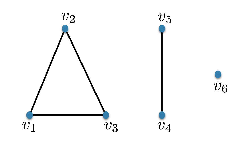
Let \(G=(V,E)\) where \[V = \{v_1,v_2,v_3,v_4,v_5,v_6\}\] and \[E = \{\{v_1,v_2\},\{v_1,v_3\},\{v_2,v_3\},\{v_4,v_5\}\}.\] We usually draw graphs in a way such that a vertex corresponds to a dot and an edge corresponds to a line connecting two dots. For example, the graph we have defined can be drawn as follows:
Given a graph \(G=(V,E)\), we usually use \(n\) to denote the number of vertices \(|V|\) and \(m\) to denote the number of edges \(|E|\).
There are two common ways to represent a graph. Let \(v_1,v_2,\ldots,v_n\) be some arbitrary ordering of the vertices. In the adjacency matrix representation, a graph is represented by an \(n \times n\) matrix \(A\) such that \[A[i,j] = \begin{cases} 1 & \quad \text{if $\{v_i,v_j\} \in E$,}\\ 0 & \quad \text{otherwise.}\\ \end{cases}\] The adjacency matrix representation is not always the best representation of a graph. In particular, it is wasteful if the graph has very few edges. For such graphs, it can be preferable to use the adjacency list representation. In the adjacency list representation, you are given an array of size \(n\) and the \(i\)’th entry of the array contains a pointer to a linked list of vertices that vertex \(i\) is connected to via an edge.
In an \(n\)-vertex graph, what is the maximum possible value for the number of edges in terms of \(n\)?
An edge is a subset of \(V\) of size \(2\), and there are at most \(n \choose 2\) possible subsets of size \(2\).
Let \(G=(V,E)\) be a graph, and \(e = \{u,v\} \in E\) be an edge in the graph. In this case, we say that \(u\) and \(v\) are neighbors or adjacent. We also say that \(u\) and \(v\) are incident to \(e\). For \(v \in V\), we define the neighborhood of \(v\), denoted \(N(v)\), as the set of all neighbors of \(v\), i.e. \(N(v) = \{u : \{v,u\} \in E\}\). The size of the neighborhood, \(|N(v)|\), is called the degree of \(v\), and is denoted by \(\deg(v)\).
Consider Example (A graph with \(6\) vertices and \(4\) edges). We have \(N(v_1) = \{v_2,v_3\}\), \(\deg(v_1) = \deg(v_2) = \deg(v_3) = 2\), \(\deg(v_4) = \deg(v_5) = 1\), and \(\deg(v_6) = 0\).
A graph \(G = (V,E)\) is called \(d\)-regular if every vertex \(v \in V\) satisfies \(\deg(v) = d\).
Our goal is to show that the sum of the degrees of all the vertices is equal to twice the number of edges. We will use a double counting argument to establish the equality. This means we will identify a set of objects and count its size in two different ways. One way of counting it will give us \(\sum_{v \in V} \deg(v)\), and the second way of counting it will give us \(2m\). This then immediately implies that \(\sum_{v \in V} \deg(v) = 2m\).
We now proceed with the double counting argument. For each vertex \(v \in V\), put a “token” on all the edges it is incident to. We want to count the total number of tokens. Every vertex \(v\) is incident to \(\deg(v)\) edges, so the total number of tokens put is \(\sum_{v \in V} \deg(v)\). On the other hand, each edge \(\{u,v\}\) in the graph will get two tokens, one from vertex \(u\) and one from vertex \(v\). So the total number of tokens put is \(2m\). Therefore it must be that \(\sum_{v \in V} \deg(v) = 2m\).
Is it possible to have a party with 251 people in which everyone knows exactly 5 other people in the party?
Create a vertex for each person in the party, and put an edge between two people if they know each other. Note that the question is asking whether there can be a \(5\)-regular graph with \(251\) nodes. We use Handshake Theorem to answer this question. If such a graph exists, then the sum of the degrees would be \(5 \times 251\), which is an odd number. However, this number must equal \(2m\) (where \(m\) is the number of edges), and \(2m\) is an even number. So we conclude that there cannot be a party with 251 people in which everyone knows exactly 5 other people.
Let \(G=(V,E)\) be a graph. A path of length \(k\) in \(G\) is a sequence of distinct vertices \[v_0,v_1,\ldots,v_k\] such that \(\{v_{i-1}, v_i\} \in E\) for all \(i \in \{1,2,\ldots,k\}\). In this case, we say that the path is from vertex \(v_0\) to vertex \(v_k\) (or that the path is between \(v_0\) and \(v_k\)).
A cycle of length \(k\) (also known as a \(k\)-cycle) in \(G\) is a sequence of vertices \[v_0, v_1, \ldots, v_{k-1}, v_0\] such that \(v_0, v_1, \ldots, v_{k-1}\) is a path, and \(\{v_0,v_{k-1}\} \in E\). In other words, a cycle is just a “closed” path. The starting vertex in the cycle is not important. So for example, \[v_1, v_2, \ldots, v_{k-1},v_0,v_1\] would be considered the same cycle. Also, if we list the vertices in reverse order, we consider it to be the same cycle. For example, \[v_0, v_{k-1}, v_{k-2} \ldots, v_1, v_0\] represents the same cycle as before.
A graph that contains no cycles is called acyclic.
Let \(G = (V,E)\) be a graph. We say that two vertices in \(G\) are connected if there is a path between those two vertices. A connected graph \(G\) is such that every pair of vertices in \(G\) is connected.
A subset \(S \subseteq V\) is called a connected component of \(G\) if \(G\) restricted to \(S\), i.e. the graph \(G' = (S, E' = \{\{u,v\} \in E : u,v \in S\})\), is a connected graph, and \(S\) is disconnected from the rest of the graph (i.e. \(\{u,v\} \not \in E\) when \(u \in S\) and \(v \not \in S\)). Note that a connected graph is a graph with only one connected component.
Let \(G=(V,E)\) be a graph. The distance between vertices \(u, v \in V\), denoted \(\text{dist}(u,v)\), is defined to be the length of the shortest path between \(u\) and \(v\). If \(u = v\), then \(\text{dist}(u,v) = 0\), and if \(u\) and \(v\) are not connected, then \(\text{dist}(u,v)\) is defined to be \(\infty\).
Let \(G = (V,E)\) be a connected graph with \(n\) vertices and \(m\) edges. Then \(m \geq n-1\). Furthermore, \(m = n-1\) if and only if \(G\) is acyclic.
We first prove that a connected graph with \(n\) vertices and \(m\) edges satisfies \(m \geq n-1\). Take \(G\) and remove all its edges. This graph consists of isolated vertices and therefore contains \(n\) connected components. Let’s now imagine a process in which we put back the edges of \(G\) one by one. The order in which we do this does not matter. At the end of this process, we must end up with just one connected component since \(G\) is connected. When we put back an edge, there are two options. Either
we connect two different connected components by putting an edge between two vertices that are not already connected, or
we put an edge between two vertices that are already connected, and therefore create a cycle.
Observe that if (1) happens, then the number of connected components goes down by 1. If (2) happens, the number of connected components remains the same. So every time we put back an edge, the number of connected components in the graph can go down by at most 1. Since we start with \(n\) connected components and end with \(1\) connected component, (1) must happen at least \(n-1\) times, and hence \(m \geq n-1\). This proves the first part of the theorem. We now prove \(m = n-1 \Longleftrightarrow \text{$G$ is acyclic}\).
\(m = n-1 \implies \text{$G$ is acyclic}\): If \(m = n-1\), then (1) must have happened at each step since otherwise, we could not have ended up with one connected component. Note that (1) cannot create a cycle, so in this case, our original graph must be acyclic.
\(\text{$G$ is acyclic} \implies m = n-1\): To prove this direction (using the contrapositive), assume \(m > n-1\). We know that (1) can happen at most \(n-1\) times. So in at least one of the steps, (2) must happen. This implies \(G\) contains a cycle.
A graph satisfying two of the following three properties is called a tree:
connected,
\(m = n-1\),
acyclic.
A vertex of degree 1 in a tree is called a leaf. And a vertex of degree more than 1 is called an internal node.
Show that if a graph has two of the properties listed in Definition (Tree, leaf, internal node), then it automatically has the third as well.
If a graph is connected and satisfies \(m = n-1\), then it must be acyclic by Theorem (Min number of edges to connect a graph). If a graph is connected and acyclic, then it must satisfy \(m = n-1\), also by Theorem (Min number of edges to connect a graph). So all we really need to prove is if a graph is acyclic and satisfies \(m=n-1\), then it is connected. For this we look into the proof of Theorem (Min number of edges to connect a graph). If the graph is acyclic, this means that every time we put back an edge, we put one that satisfies (1) (here “(1)” is referring to the item in the proof of Theorem (Min number of edges to connect a graph)). This is because any edge that satisfies (2) creates a cycle. Every time we put an edge satisfying (1), we reduce the number of connected components by 1. Since \(m = n-1\), we put back \(n-1\) edges. This means we start with \(n\) connected components (\(n\) isolated vertices), and end up with \(1\) connected component once all the edges are added back. So the graph is connected.
Let \(T\) be a tree with at least \(2\) vertices. Show that \(T\) must have at least \(2\) leaves.
We use Handshake Theorem to prove this (i.e. \(\sum_v \deg(v) = 2m\)). We’ll go by contradiction, so assume there is some tree \(T\) with \(n \geq 2\) and less than 2 leaves. Note that in any tree we have \(m = n-1\), and so \(\sum_v \deg(v) = 2m = 2(n-1) = 2n-2\). On the other hand, for a tree with at most one leaf, let’s calculate the minimum value that \(\sum_v \deg(v)\) can have. The minimum value would be obtained if there was 1 leaf and the other \(n-1\) vertices all had degree \(2\). In this case, the sum of the degrees of the vertices would be \[1 + 2(n-1) = 2n - 1.\] Putting things together, we have \(2n-2 = \sum_v \deg(v) \geq 2n-1\). This is the desired contradiction.
Let \(T\) be a tree with \(L\) leaves. Let \(\Delta\) be the largest degree of any vertex in \(T\). Prove that \(\Delta \leq L\).
It is instructive to read all 3 proofs.
Proof 1: We use Handshake Theorem. The degree sum in a tree is always \(2n - 2\) since \(m = n-1\). Let \(v\) be the vertex with maximum degree \(\Delta\). The vertices that are not \(v\) or leaves must have degree at least \(2\) each, so the degree sum is at least \(\deg(v) + L + 2(n - L - 1)\). So we must have \(2n - 2 \geq \deg(v) + L + 2(n - L - 1)\), which simplifies to \(L \geq \deg(v) = \Delta\), as desired.
Proof 2: We induct on the number of vertices. For \(n \leq 3\), this follows by inspecting the unique tree on \(n\) vertices. For \(n > 3\), pick an arbitrary leaf \(u\) and delete it (and the edge incident to \(u\)). Let \(T - u\) denote this graph, which is a tree (it is connected and acyclic). Also, we let \(L(T)\) denote the number of leaves in \(T\) and \(L(T-u)\) to denote the number of leaves in \(T-u\). We make similar definitions for \(\Delta(T)\) and \(\Delta(T-u)\) regarding the maximum degrees. Note that \(L(T) \geq L(T - u)\). There are two cases to consider:
\(\Delta(T - u) = \Delta(T)\)
\(\Delta(T - u) = \Delta(T) - 1\)
If case 1 happens, then by the induction hypothesis \(L(T - u) \geq \Delta(T-u) = \Delta(T)\). But this implies \(L(T) \geq \Delta(T)\) (since \(L(T) \geq L(T - u)\)), as desired.
Let \(v\) be the neighbor of \(u\). If case 2 happens, then \(v\) is the only vertex of maximum degree in \(T\). In particular, \(v\) cannot be a leaf in \(T-u\). So \(L(T) = L(T - u) + 1\). The induction hypothesis yields \(L(T - u) \geq \Delta(T-u) = \Delta(T) - 1\). Combining this with \(L(T) = L(T - u) + 1\) we get \(L(T) \geq \Delta(T)\), as desired.
Proof 3: Let \(v\) be a vertex in the tree such that \(\deg(v) = \Delta.\) Consider the graph \(T - v\) obtained by deleting \(v\) and all the edges incident to it. Since \(T\) is a tree, we know that \(T-v\) contains \(\Delta\) connected components; let us denote them \(T_1,\ldots, T_{\Delta}\). Since \(T\) is acyclic, each of the \(T_i\)’s are also acyclic. Since each \(T_i\) is connected and acyclic, each one is a tree. There are two possibilities for each \(T_i\):
\(T_i\) consists of a single vertex. Then that vertex is a leaf in \(T\).
\(T_i\) is not a single vertex, and so has at least \(2\) leaves (by Exercise (A tree has at least 2 leaves)). At least one of these leaves is not a neighbor of \(v\) and therefore must be a leaf in \(T\).
In either case, one vertex in \(T_i\) is a leaf in \(T\). This is true for all \(T_1, \ldots, T_{\Delta}\). Hence we have at least \(\Delta\) leaves in \(T\).
Given a tree, we can pick an arbitrary node to be the root of the tree. In a rooted tree, we use “family tree” terminology: parent, child, sibling, ancestor, descendant, lowest common ancestor, etc. (We assume you are already familiar with these terms.) Level \(i\) of a rooted tree denotes the set of all vertices in the tree at distance \(i\) from the root.
A directed graph \(G\) is a pair \((V,A)\), where
\(V\) is a non-empty finite set called the set of vertices (or nodes),
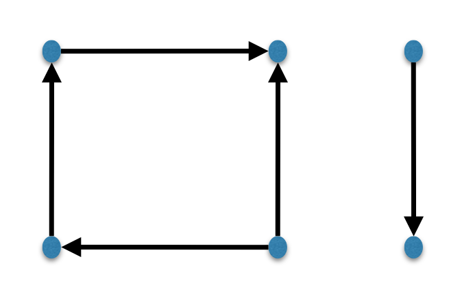
\(A\) is a finite set called the set of directed edges (or arcs), and every element of \(A\) is a tuple \((u,v)\) for \(u, v \in V\). If \((u,v) \in A\), we say that there is a directed edge from \(u\) to \(v\). Note that \((u,v) \neq (v,u)\) unless \(u = v\).
Below is an example of how we draw a directed graph:
Let \(G = (V,A)\) be a directed graph. For \(u \in V\), we define the neighborhood of \(u\), \(N(u)\), as the set \(\{v \in V : (u,v) \in A\}\). The vertices in \(N(u)\) are called the neighbors of \(u\). The out-degree of \(u\), denoted \(\deg_\text{out}(u)\), is \(|N(u)|\). The in-degree of \(u\), denoted \(\deg_\text{in}(u)\), is the size of the set \(\{v \in V : (v,u) \in A\}\). A vertex with out-degree 0 is called a sink. A vertex with in-degree 0 is called a source.
The notions of paths and cycles naturally extend to directed graphs. For example, we say that there is a path from \(u\) to \(v\) if there is a sequence of distinct vertices \(u = v_0,v_1,\ldots,v_k = v\) such that \((v_{i-1}, v_i) \in A\) for all \(i \in \{1,2,\ldots,k\}\).
The arbitrary-first search algorithm, denoted AFS, is the following generic algorithm for searching a given graph. Below, “bag” refers to an arbitrary data structure that allows us to add and retrieve objects. The algorithm, given a graph \(G\) and some vertex \(s\) in \(G\), traverses all the vertices in the connected componenet of \(G\) containing \(s\).
\[\begin{aligned} \hline\hline\\[-12pt] &\textbf{def}\;\; \text{AFS}(\langle \text{graph } G = (V,E), \; \text{vertex } s \in V \rangle):\\ &{\scriptstyle 1.}~~~~\texttt{Put $s$ into bag.}\\ &{\scriptstyle 2.}~~~~\texttt{While bag is non-empty:}\\ &{\scriptstyle 3.}~~~~~~~~\texttt{Pick an arbitrary vertex $v$ from bag.}\\ &{\scriptstyle 4.}~~~~~~~~\texttt{If $v$ is unmarked:}\\ &{\scriptstyle 5.}~~~~~~~~~~~~\texttt{Mark $v$.}\\ &{\scriptstyle 6.}~~~~~~~~~~~~\texttt{For each neighbor $w$ of $v$:}\\ &{\scriptstyle 7.}~~~~~~~~~~~~~~~~\texttt{Put $w$ into bag.}\\ \hline\hline\end{aligned}\]
Note that when a vertex \(w\) is added to the bag, it gets there because it is the neighbor of a vertex \(v\) that has been just marked by the algorithm. In this case, we’ll say that \(v\) is the parent of \(w\) (and \(w\) is the child of \(v\)). Explicitly keeping track of this parent-child relationship is convenient, so we modify the above algorithm to keep track of this information. Below, a tuple of vertices \((v,w)\) has the meaning that vertex \(v\) is the parent of \(w\). The initial vertex \(s\) has no parent, so we denote this situation by \((\perp, s)\).
\[\begin{aligned} \hline\hline\\[-12pt] &\textbf{def}\;\; \text{AFS}(\langle \text{graph } G = (V,E), \; \text{vertex } s \in V \rangle):\\ &{\scriptstyle 1.}~~~~\texttt{Put $(\perp, s)$ into bag.}\\ &{\scriptstyle 2.}~~~~\texttt{While bag is non-empty:}\\ &{\scriptstyle 3.}~~~~~~~~\texttt{Pick an arbitrary tuple $(p, v)$ from bag.}\\ &{\scriptstyle 4.}~~~~~~~~\texttt{If $v$ is unmarked:}\\ &{\scriptstyle 5.}~~~~~~~~~~~~\texttt{Mark $v$.}\\ &{\scriptstyle 6.}~~~~~~~~~~~~\text{parent}(v) = p.\\ &{\scriptstyle 7.}~~~~~~~~~~~~\texttt{For each neighbor $w$ of $v$:}\\ &{\scriptstyle 8.}~~~~~~~~~~~~~~~~\texttt{Put $(v,w)$ into bag.}\\ \hline\hline\end{aligned}\]
The parent pointers in the second algorithm above defines a tree, rooted at \(s\), spanning all the vertices in the connected component of the initial vertex \(s\). We’ll call this the tree induced by the search algorithm. Having a visualization of this tree and how the algorithm traverses the vertices in the tree can be a useful way to understand how the algorithm works. Below, we will actualize AFS by picking specific data structures for the bag. We’ll then comment on the properties of the induced tree.
Note that AFS(\(G\), \(s\)) visits all the vertices in the connected component that \(s\) is a part of. If we want to traverse all the vertices in the graph, and the graph has multiple connected components, then we can do: \[\begin{aligned} \hline\hline\\[-12pt] &\textbf{def}\;\; \text{AFS2}(\langle \text{graph } G = (V,E) \rangle):\\ &{\scriptstyle 1.}~~~~\texttt{For $v$ not marked as visited:}\\ &{\scriptstyle 2.}~~~~~~~~\texttt{Run } \text{AFS}(\langle G, v \rangle)\\ \hline\hline\end{aligned}\]
The breadth-first search algorithm, denoted BFS, is AFS where the bag is chosen to be a queue data structure.
The induced tree of BFS is called the BFS-tree. In this tree, vertices \(v\) at level \(i\) of the tree are exactly those vertices with \(\text{dist}(s,v) = i\). BFS first traverses vertices at level 1, then level 2, then level 3, and so on. This is why the name of the algorithm is breadth-first search.
Assuming \(G\) is connected, we can think of \(G\) as the BFS-tree, plus, the “extra” edges in \(G\) that are not part of the BFS-tree. Observe that an extra edge is either between two vertices at the same level, or is between two vertices at consecutive levels.
The depth-first search algorithm, denoted DFS, is AFS where the bag is chosen to be a stack data structure.
There is a natural recursive representation of the DFS algorithm, as follows. \[\begin{aligned} \hline\hline\\[-12pt] &\textbf{def}\;\; \text{DFS}(\langle \text{graph } G = (V,E), \; \text{vertex } s \in V \rangle):\\ &{\scriptstyle 1.}~~~~\texttt{Mark $s$.}\\ &{\scriptstyle 2.}~~~~\texttt{For each neighbor $v$ of $s$:}\\ &{\scriptstyle 3.}~~~~~~~~\texttt{If $v$ is unmarked:}\\ &{\scriptstyle 4.}~~~~~~~~~~~~\texttt{Run } \text{DFS}(\langle G, v \rangle).\\ \hline\hline\end{aligned}\]
The running time of DFS(\(G,s\)) is \(O(m)\), where \(m\) is the number of edges of the input graph. If we do a DFS for each connected component, the total running time is \(O(m+n)\), where \(n\) is the number of vertices. (We are assuming the graph is given as an adjacency list.)
The induced tree of DFS is called the DFS-tree. At a high level, DFS goes as deep as it can in the DFS-tree until it cannot go deeper, in which case it backtracks until it can go deeper again. This is why the name of the algorithm is depth-first search.
Assuming \(G\) is connected, we can think of \(G\) as the DFS-tree, plus, the “extra” edges in \(G\) that are not part of the DFS-tree. Observe that an extra edge must be between two vertices such that one is the ancestor of the other.
The search algorithms presented above can be applied to directed graphs as well.
In the minimum spanning tree problem, the input is a connected undirected graph \(G = (V,E)\) together with a cost function \(c : E \to \mathbb R^+\). The output is a subset of the edges of minimum total cost such that, in the graph restricted to these edges, all the vertices of \(G\) are connected. For convenience, we’ll assume that the edges have unique edge costs, i.e. \(e \neq e' \implies c(e) \neq c(e')\).
With unique edge costs, the minimum spanning tree is unique.
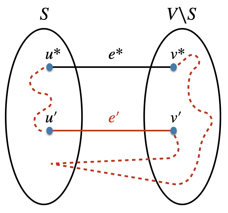
Suppose we are given an instance of the MST problem. For any non-trivial subset \(S \subseteq V\), let \(e^* = \{u^*, v^*\}\) be the cheapest edge with the property that \(u^* \in S\) and \(v^* \in V \backslash S\). Then \(e^*\) must be in the minimum spanning tree.
The overall proof strategy is to show that if \(e^*\) is not in the MST, then we can find an edge \(e' = \{u',v'\}\) from the MST (with \(u' \in S\) and \(v' \in V \backslash S\)) such that replacing \(e'\) with \(e^*\) in the MST results in a new spanning tree with a smaller cost, a contradiction. We now flesh this out.
Let \(T\) be the minimum spanning tree. The proof is by contradiction, so assume that \(e^* = \{u^*,v^*\}\) is not in \(T\). Since \(T\) spans the whole graph, there must be a path from \(u^*\) to \(v^*\) in \(T\). Let \(e' = \{u',v'\}\) be the first edge on this path such that \(u' \in S\) and \(v' \in V \backslash S\). Let \(T^* = (T \backslash \{e'\}) \cup \{e^*\}\). If \(T^*\) is a spanning tree, then we reach a contradiction because \(T^*\) has lower cost than \(T\) (since \(c(e^*) < c(e')\)).
We now show that \(T^*\) is a spanning tree. Clearly \(T^*\) has \(n-1\) edges (since \(T\) has \(n-1\) edges). So if we can show that \(T^*\) is connected, this would imply that \(T^*\) is a tree and touches every vertex of the graph, i.e., \(T^*\) is a spanning tree.
To conclude the proof, we’ll now show that \(T^*\) is connected. Consider any two vertices \(s,t \in V\). We want to show that we can reach \(t\) starting from \(s\). We know there is a unique path from \(s\) to \(t\) in \(T\). If this path does not use the edge \(e' = \{u',v'\}\), then the same path exists in \(T^*\), so \(s\) and \(t\) are connected in \(T^*\). If the path does use \(e' = \{u',v'\}\), then instead of taking the edge \(\{u',v'\}\), we can take the following path: take the path from \(u'\) to \(u^*\), then take the edge \(e^* = \{u^*,v^*\}\), then take the path from \(v^*\) to \(v'\). So replacing \(\{u',v'\}\) with this path allows us to construct a sequence of vertices starting from \(s\) and ending at \(t\), such that each consecutive pair of vertices is an edge. Therefore, \(s\) and \(t\) are connected.
There is an algorithm that solves the MST problem in polynomial time.
We first present the algorithm which is due to Jarník and Prim. Given an undirected graph \(G=(V,E)\) and a cost function \(c : E \to \mathbb R^+\): \[\begin{aligned} \hline\hline\\[-12pt] &\textbf{def}\;\; \text{MST}(\langle \text{graph } G = (V,E), \; \text{function } c:E \to \mathbb{R}^+ \rangle):\\ &{\scriptstyle 1.}~~~~\texttt{$V' = \{u\}$ (for some arbitrary $u \in V$).}\\ &{\scriptstyle 2.}~~~~\texttt{$E' = \varnothing$.}\\ &{\scriptstyle 3.}~~~~\texttt{While $V' \neq V$:}\\ &{\scriptstyle 4.}~~~~~~~~\texttt{Let $\{u,v\}$ be the min cost edge such that $u \in V'$ but $v \not\in V'$.}\\ &{\scriptstyle 5.}~~~~~~~~\texttt{Add $\{u,v\}$ to $E'$.}\\ &{\scriptstyle 6.}~~~~~~~~\texttt{Add $v$ to $V'$.}\\ &{\scriptstyle 7.}~~~~\texttt{Return $E'$.}\\ \hline\hline\end{aligned}\]
By Theorem (MST cut property), the algorithm always adds an edge that must be in the MST. The number of iterations is \(n-1\), so all the edges of the MST are added to \(E'\). Therefore the algorithm correctly outputs the unique MST.
The running time of the algorithm can be upper bounded by \(O(nm)\) because there are \(O(n)\) iterations, and the body of the loop can be done in \(O(m)\) time.
Suppose an instance of the Minimum Spanning Tree problem is allowed to have negative costs for the edges. Explain whether we can use the Jarník-Prim algorithm to compute the minimum spanning tree in this case.
Yes, we can. Assign a rank to each edge of the graph based on its cost: the highest cost edge gets the highest rank and the lowest cost edge gets the lowest rank. When making its decisions, the Jarník-Prim algorithm only cares about the ranks of the edges, and not the specific costs of the edges. The algorithm would output the same tree even if we add a constant \(C\) to the costs of all the edges since this would not change the rank of the edges. And indeed, adding a constant to the cost of each edge does not change what the minimum spanning tree is. Hence, we can turn any instance with negative costs into and equivalent one with non-negative costs by adding a large enough constant to all the edges without changing the tree that is output.
(Note: In fact the original algorithm would output the minimum cost spanning tree even if the edge costs are allowed to be negative. There is not even a need to add a constant to the edge costs.)
Consider the problem of computing the maximum spanning tree, i.e., a spanning tree that maximizes the sum of the edge costs. Explain whether the Jarník-Prim algorithm solves this problem if we modify it so that at each iteration, the algorithm chooses the edge between \(V'\) and \(V\backslash V'\) with the maximum cost.
Let \((G,c)\) be the input, where \(G = (V,E)\) is a graph and \(c: E \to \mathbb{R}^+\) is the cost function. Let \(c' : E \to \mathbb{R}^{-}\) be defined as follows: for all \(e \in E\), \(c'(e) = - c(e)\). Let \(A_{\min}\) be the original Jarník-Prim algorithm and let \(A_{\max}\) be the Jarník-Prim algorithm where we pick the maximum cost edge in each iteration. There are a couple of important observations:
The minimum spanning tree for \((G,c')\) is the maximum spanning tree for \((G,c)\).
Running \(A_{\max}(G,c)\) is equivalent to running \(A_{\min}(G,c')\), and they output the same spanning tree.
From Exercise (MST with negative costs), we know \(A_{\min}(G,c')\) gives us a minimum cost spanning tree. So \(A_{\max}(G,c)\) gives the correct maximum cost spanning tree.
What is the maximum possible value for the number of edges in an undirected graph (no self-loops, no multi-edges) in terms of \(n\), the number of vertices?
How do you prove the Handshake Theorem?
What is the definition of a tree?
True or false: If \(G = (V, E)\) is a tree, then for any \(u, v \in V\), there exists a unique path from \(u\) to \(v\).
True or false: For a graph \(G = (V, E)\), if for any \(u, v \in V\) there exists a unique path from \(u\) to \(v\), then \(G\) is a tree.
True or false: If a graph on \(n\) vertices has \(n-1\) edges, then it must be acyclic.
True or false: If a graph on \(n\) vertices has \(n-1\) edges, then it must be connected.
True or false: If a graph on \(n\) vertices has \(n-1\) edges, then it must be a tree.
True or false: A tree with \(n \geq 2\) vertices can have a single leaf.
What is the minimum number of edges possible in a connected graph with \(n\) vertices? And what are the high-level steps of the proof?
True or false: An acyclic graph with \(k\) connected components has \(n-k\) edges.
True or false: For every tree on \(n\) vertices, \(\sum_{v \in V} \deg(v)\) has exactly the same value.
True or false: Let \(G\) be a \(5\)-regular graph (i.e. a graph in which every vertex has degree exactly \(5\)). It is possible that \(G\) has \(15251\) edges.
True or false: There exists \(n_0 \in \mathbb{N}\) such that for all \(n > n_0\), there is a graph \(G\) with \(n\) vertices that is \(3\)-regular.
What is the difference between BFS and DFS?
True or false: DFS algorithm runs in \(O(n)\) time for a connected graph, where \(n\) is the number of vertices of the input graph.
Explain why the running time of BFS and DFS is \(O(m+n)\); in particular where does the \(m\) come from and where does the \(n\) come from?
What is the MST cut property?
Explain at a high-level how the Jarník-Prim algorithm works.
True or false: Suppose a graph has \(2\) edges with the same cost. Then there are at least \(2\) minimum spanning trees of the graph.
Here are the important things to keep in mind from this chapter.
There are many definitions in this chapter. This is unfortunately inevitable in order to effectively communicate with each other. On the positive side, the definitions are often very intuitive and easy to guess. It is important that you are comfortable with all the definitions.
In the first section of the chapter, we see a few proof techniques on graphs: degree counting arguments, induction arguments, the trick of removing all the edges of graph and adding them back in one by one. Make sure you understand these techniques well. They can be very helpful when you are coming up with proofs yourself.
The second section of the chapter contains some well-known graph algorithms. These algorithms are quite fundamental, and you may have seen them (or will see them) in other courses. Make sure you understand at a high level how the algorithms work. The implementation details are not important in this course.