Polynomial-Time Reductions | Text

MODULE 8: P vs NP

Polynomial-Time Reductions

In a previous chapter, we have studied reductions and saw how they can be used to both expand the landscape of decidable languages and expand the landscape of undecidable languages. As such, the concept of a reduction is a very powerful tool.

In the context of computational complexity, reductions once again play a very important role. In particular, by tweaking our definition of a reduction a bit so that it is required to be efficiently computable, we can use reductions to expand the landscape of tractable (i.e. efficiently decidable) languages and to expand the landscape of intractable languages. Another cool feature of reductions is that it allows us to show that many seemingly unrelated problems are essentially the same problem in disguise, and this allows us to have a deeper understanding of the mysterious and fascinating world of computational complexity.

Our goal in this chapter is to introduce you to the concept of polynomial-time (efficient) reductions, and give you a few examples to make the concept more concrete and illustrate their power.

In some sense, this chapter marks the introduction to our discussion on the $\mathsf{P}$ vs $\mathsf{NP}$ problem, even though the definition of $\mathsf{NP}$ will only be introduced in the next chapter, and the connection will be made more precise then.

1 Problems of Interest

In this section, we present the definitions of some of the decision problems that will be part of our discussion in this module.

Definition (

k

-Coloring problem)

In the $k$ -coloring problem, the input is an undirected graph $G=(V,E)$ , and the output is True if and only if the graph is $k$ -colorable (see Definition ( $k$ -colorable graphs)). We denote this problem by $k\text{COL}$ . The corresponding language is $\{\langle G \rangle: \text{$G$ is a $k$-colorable graph}\}.$

Definition (Clique problem)

Let $G = (V,E)$ be an undirected graph. A subset $S$ of the vertices is called a clique if for all $u, v \in S$ with $u \neq v$ , $\{u,v\} \in E$ . We say that $G$ contains a $k$ -clique if there is a subset of the vertices of size $k$ that forms a clique.

In the clique problem, the input is an undirected graph $G=(V,E)$ and a number $k \in \mathbb N^+$ , and the output is True if and only if the graph contains a $k$ -clique. We denote this problem by $\text{CLIQUE}$ . The corresponding language is $\{\langle G, k \rangle: \text{$G$ is a graph, $k \in \mathbb N^+$, $G$ contains a $k$-clique}\}.$

Definition (Independent set problem)

Let $G = (V,E)$ be an undirected graph. A subset of the vertices is called an independent set if there is no edge between any two vertices in the subset. We say that $G$ contains an independent set of size $k$ if there is a subset of the vertices of size $k$ that forms an independent set.

In the independent set problem, the input is an undirected graph $G=(V,E)$ and a number $k \in \mathbb N^+$ , and the output is True if and only if the graph contains an independent set of size $k$ . We denote this problem by $\text{IS}$ . The corresponding language is $\{\langle G, k \rangle: \text{$G$ is a graph, $k \in \mathbb N^+$, $G$ contains an independent set of size $k$}\}.$

Note (Unary NOT, binary AND, binary OR)

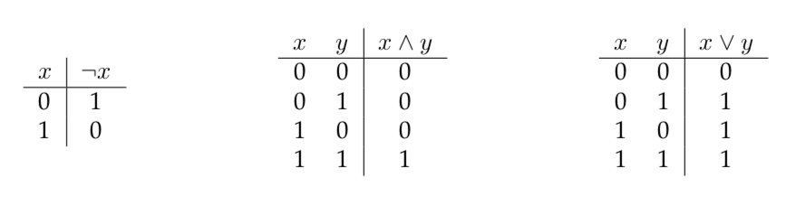
We denote by $\neg$ the unary NOT operation, by $\wedge$ the binary AND operation, and by $\vee$ the binary OR operation. In particular, we can write the truth tables of these operations as follows:

Definition (Boolean satisfiability problem)

Let $x_1,\ldots,x_n$ be Boolean variables, i.e., variables that can be assigned True or False. A literal refers to a Boolean variable or its negation. A clause is an “OR” of literals. For example, $x_1 \vee \neg x_3 \vee x_4$ is a clause. A Boolean formula in conjunctive normal form (CNF) is an “AND” of clauses. For example, $(x_1 \vee \neg x_3) \wedge (x_2 \vee x_2 \vee x_4) \wedge (x_1 \vee \neg x_1 \vee \neg x_5) \wedge x_4$ is a CNF formula. We say that a Boolean formula is a satisfiable formula if there is a truth assignment (which can also be viewed as a $0/1$ assignment) to the Boolean variables that makes the formula evaluate to true (or $1$ ).

In the CNF satisfiability problem, the input is a CNF formula, and the output is True if and only if the formula is satisfiable. We denote this problem by $\text{SAT}$ . The corresponding language is $\{\langle \varphi \rangle: \text{$\varphi$ is a satisfiable CNF formula}\}.$ In a variation of $\text{SAT}$ , we restrict the input formula such that every clause has exactly 3 literals (we call such a formula a 3CNF formula). For instance, the following is a 3CNF formula: For example, $(x_1 \vee \neg x_3 \vee x_4) \wedge (x_2 \vee x_2 \vee x_4) \wedge (x_1 \vee \neg x_1 \vee \neg x_5) \wedge (\neg x_2 \vee \neg x_3 \vee \neg x_3)$ This variation of the problem is denoted by $\text{3SAT}$ .

Definition (Boolean circuit)

A Boolean circuit with $n$ -input variables ( $n \geq 0$ ) is a directed acyclic graph with the following properties. Each node of the graph is called a gate and each directed edge is called a wire. There are $5$ types of gates that we can choose to include in our circuit: AND gates, OR gates, NOT gates, input gates, and constant gates. There are 2 constant gates, one labeled $0$ and one labeled $1$ . These gates have in-degree/fan-in $0$ . There are $n$ input gates, one corresponding to each input variable. These gates also have in-degree/fan-in $0$ . An AND gate corresponds to the binary AND operation $\wedge$ and an OR gate corresponds to the binary OR operation $\vee$ . These gates have in-degree/fan-in $2$ . A NOT gate corresponds to the unary NOT operation $\neg$ , and has in-degree/fan-in $1$ . One of the gates in the circuit is labeled as the output gate. Gates can have out-degree more than $1$ , except for the output gate, which has out-degree $0$ .

For each 0/1 assignment to the input variables, the Boolean circuit produces a one-bit output. The output of the circuit is the output of the gate that is labeled as the output gate. The output is calculated naturally using the truth tables of the operations corresponding to the gates. The input-output behavior of the circuit defines a function $f:\{0,1\}^n \to \{0,1\}$ and in this case, we say that $f$ is computed by the circuit.

Example

Below is an example of how we draw a circuit. In this example, $n = 4$ .

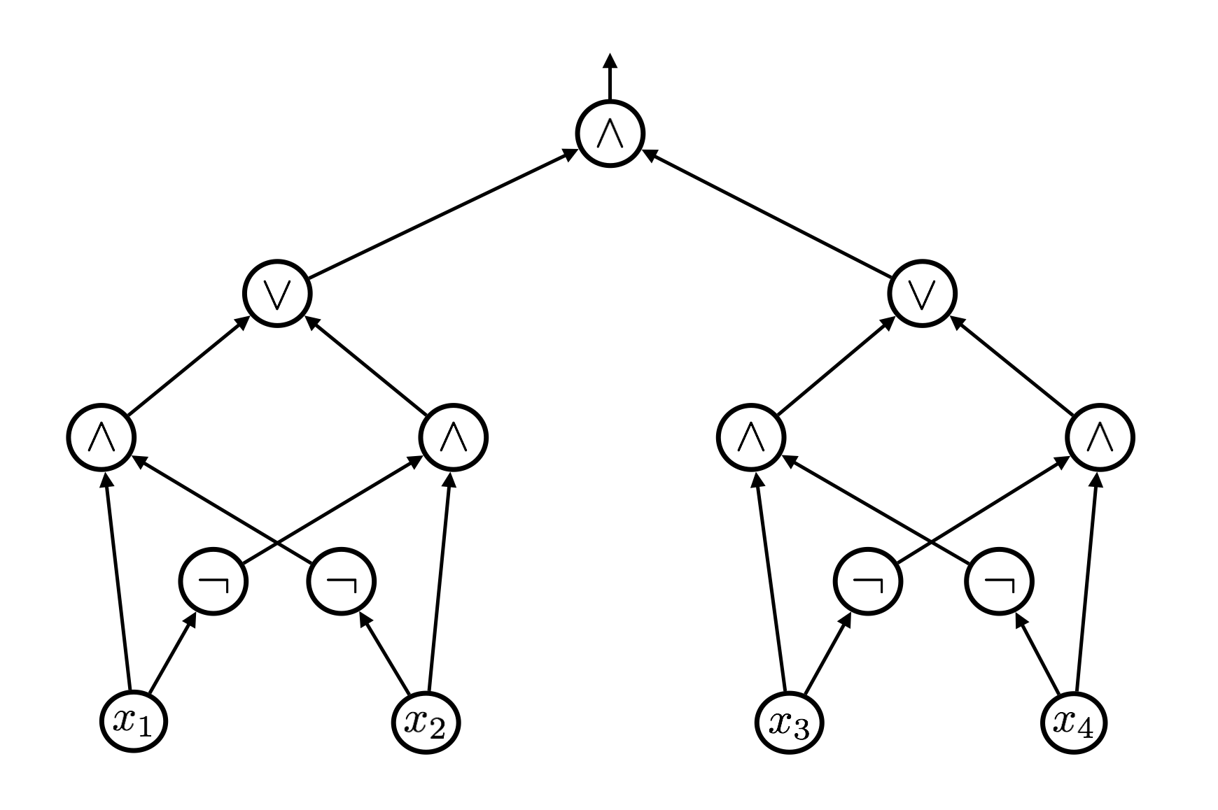
The output gate is the gate at the very top with an arrow that links to nothing. The circuit outputs 1 if and only if $x_1 \neq x_2$ and $x_3 \neq x_4$ .

Definition (Circuit satisfiability problem)

A satisfiable circuit is such that there is 0/1 assignment to the input gates that makes the circuit output 1. In the circuit satisfiability problem, the input is a Boolean circuit, and the output is True if and only if the circuit is satisfiable. We denote this problem by $\text{CIRCUIT-SAT}$ . The corresponding language is $\{\langle C \rangle: \text{$C$ is a Boolean circuit that is satisfiable}\}.$

Note (Names of decision problems and languages)

The name of a decision problem above refers both to the decision problem and the corresponding language.

Note (Inputs of decision problems)

Recall that in all the decision problems above, the input is an arbitrary word in $\Sigma^*$ . If the input does not correspond to a valid encoding of an object expected as input (e.g. a graph in the case of $k$ COL), then those inputs are rejected (i.e., they are not in the corresponding language).

Note (Exponential-time algorithms for the decision problems above)

All the problems defined above are decidable and have exponential-time algorithms solving them.

2 Cook and Karp Reductions

Note (Cook reduction: Polynomial-time (Turing) reduction)

Fix some alphabet $\Sigma$ . Let $A$ and $B$ be two languages. We say that $A$ polynomial-time reduces to $B$ , written $A \leq^PB$ , if there is a polynomial-time decider for $A$ that uses a decider for $B$ as a black-box subroutine. Polynomial-time reductions are also known as Cook reductions, named after Stephen Cook.

Note (Polynomial-time reductions and

\mathsf{P}

)

Suppose $A \leq^PB$ . Observe that if $B \in \mathsf{P}$ , then $A \in \mathsf{P}$ . Equivalently, taking the contrapositive, if $A \not \in \mathsf{P}$ , then $B \not \in \mathsf{P}$ . So when $A \leq^PB$ , we think of $B$ as being at least as hard as $A$ with respect to polynomial-time decidability.

Note (Transitivity of Cook reductions)

Note that if $A \leq^PB$ and $B \leq^PC$ , then $A \leq^PC$ .

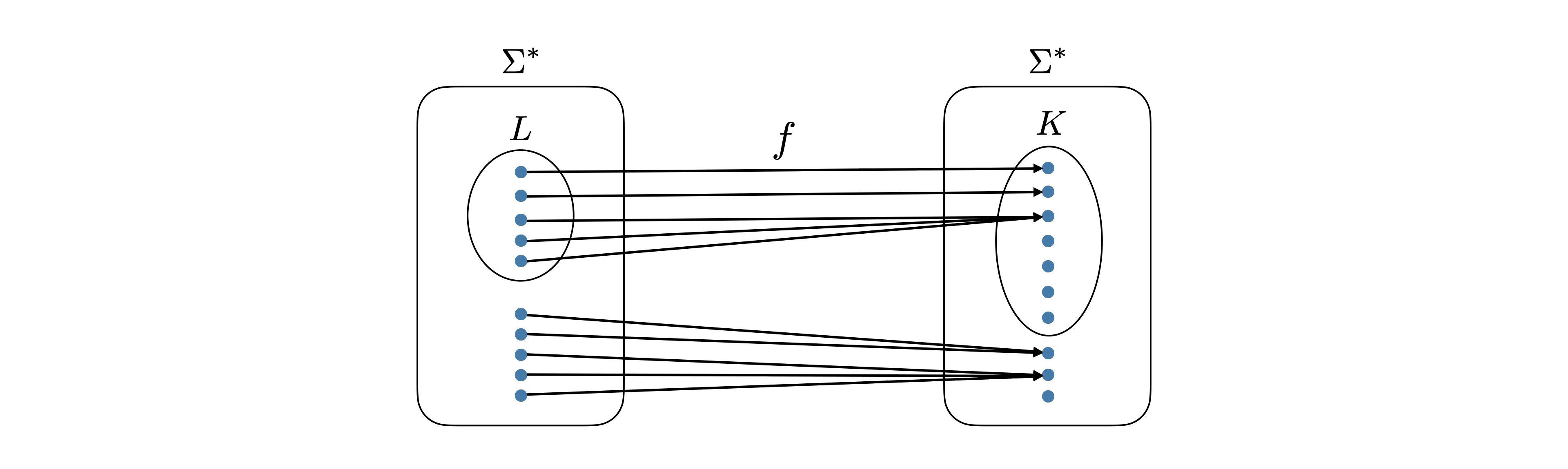
Recall that in a previous chapter, we introduced the concept of a mapping reduction (see Note (Mapping reductions)) as a special kind of a regular (Turing) reduction. We observed that to specify a mapping reduction from $L$ to $K$ , one simply needs to define an algorithm computing a function $f: \Sigma^* \to \Sigma^*$ such that $x \in L$ if and only if $f(x) \in K$ . Below we define the notion of a polynomial-time mapping reduction.

Definition (Karp reduction: Polynomial-time mapping reduction)

Let $A$ and $B$ be two languages. Suppose that there is a polynomial-time computable function (also called a polynomial-time transformation) $f: \Sigma^* \to \Sigma^*$ such that $x \in A$ if and only if $f(x) \in B$ . Then we say that there is a polynomial-time mapping reduction (or a Karp reduction, named after Richard Karp) from $A$ to $B$ , and denote it by $A \leq_m^PB$ .

Important Note (Steps to establish a Karp reduction)

To show that there is a Karp reduction from $A$ to $B$ , you need to do the following things.

Present a computable function $f: \Sigma^* \to \Sigma^*$ .
Show that $x \in A \implies f(x) \in B$ .
Show that $x \not \in A \implies f(x) \not \in B$ (it is usually easier to argue the contrapositive).
Show that $f$ can be computed in polynomial time.

In picture, the transformation $f$ looks as follows.

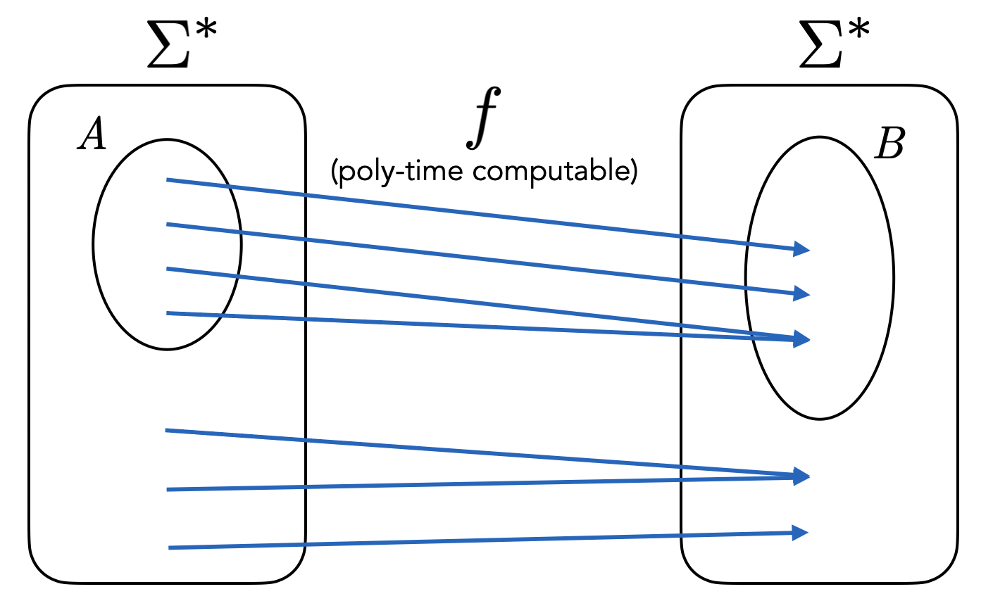
Note that $f$ need not be injective and it need not be surjective.

Important Note (Mapping reductions vs Turing reductions)

Recall that a mapping reduction is really a special kind of a Turing reduction. In particular, if there is a mapping reduction from language $A$ to language $B$ , then one can construct a regular (Turing) reduction from $A$ to $B$ . We explain this below as a reminder.

To establish a Turing reduction from $A$ to $B$ , we need to show how we can come up with a decider $M_A$ for $A$ given that we have a decider $M_B$ for $B$ . Now suppose we have a mapping reduction from $A$ to $B$ . This means we have a computable function $f$ as in the definition of a mapping reduction. This $f$ then allows us to build $M_A$ as follows. Given any input $x$ , first feed $x$ into $f$ , and then feed the output $y = f(x)$ into $M_B$ . The output of $M_A$ is the output of $M_B$ . We illustrate this construction with the following picture.

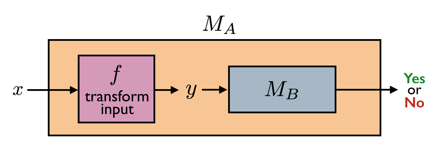
Take a moment to verify that this reduction from $A$ to $B$ is indeed correct given the definition of $f$ .

Even though a mapping reduction can be viewed as a regular (Turing) reduction, not all reductions are mapping reductions.

Theorem (CLIQUE reduces to IS)

$\text{CLIQUE} \leq_m^P\text{IS}$ .

Proof

Following the previous important note, we start by presenting a computable function $f: \Sigma^* \to \Sigma^*$ .

$\begin{aligned} \hline\hline\\[-12pt] &\textbf{def}\;\; f(\langle \text{graph } G = (V,E), \; \text{positive natural } k\rangle):\\ &{\scriptstyle 1.}~~~~\texttt{$E' = \{\{u,v\} : \{u,v\} \not\in E\}$.}\\ &{\scriptstyle 2.}~~~~\texttt{Return $\langle G' = (V,E'), k \rangle$.}\\ \hline\hline\end{aligned}$

(In a Karp reduction from $A$ to $B$ , when we define $f: \Sigma^* \to \Sigma^*$ , it is standard to define it so that invalid instances of $A$ are mapped to invalid instances of $B$ . We omit saying this explicitly when presenting the reduction, but you should be aware that this is implicitly there in the definition of $f$ . In the above definition of $f$ , for example, any string $x$ that does not correspond to a valid instance of CLIQUE (i.e., not a valid encoding of a graph $G$ together with a positive integer $k$ ) is mapped to an invalid instance of IS (e.g. they can be mapped to $\epsilon$ , which we can assume to not be a valid instance of IS.))

To show that $f$ works as desired, we first make a definition. Given a graph $G=(V,E)$ , the complement of $G$ is the graph $G' = (V,E')$ where $E' = \{\{u,v\} : \{u,v\} \not \in E\}$ . In other words, we construct $G'$ by removing all the edges of $G$ and adding all the edges that were not present in $G$ .

We now argue that $x \in \text{CLIQUE}$ if and only if $f(x) \in \text{IS}$ . First, assume $x \in \text{CLIQUE}$ . Then $x$ corresponds to a valid encoding $\langle G=(V,E), k \rangle$ of a graph and an integer. Furthermore, $G$ contains a clique $S \subseteq V$ of size $k$ . In the complement graph, this $S$ is an independent set ( $\{u,v\} \in E$ for all distinct $u,v \in S$ implies $\{u,v\} \not \in E'$ for all distinct $u,v \in S$ ). Therefore $\langle G'=(V,E'), k \rangle \in \text{IS}$ . Conversely, if $\langle G'=(V,E'), k \rangle \in \text{IS}$ , then $G'$ contains an independent set $S \subseteq V$ of size $k$ . This set $S$ is a clique in the complement of $G'$ , which is $G$ . So the pre-image of $\langle G'=(V,E'), k \rangle$ under $f$ , which is $\langle G=(V,E), k \rangle$ , is in CLIQUE.

Finally, we argue that the function $f$ can be computed in polynomial time. This is easy to see since the construction of $E'$ (and therefore $G'$ ) can be done in polynomial time as there are polynomially many possible edges.

Exercise (IS reduces to CLIQUE)

How can you modify the above reduction to show that $\text{IS} \leq_m^P\text{CLIQUE}$ ?

Solution

We can use exactly the same reduction as the one in the reduction from CLIQUE to IS:

This reduction establishes $\text{IS} \leq_m^P\text{CLIQUE}$ . The proof of correctness is the same as in the proof of Theorem (CLIQUE reduces to IS); just interchange the words “clique” and “independent set” in the proof.

Exercise (Hamiltonian path reductions)

Let $G=(V,E)$ be a graph. A Hamiltonian path in $G$ is a path that visits every vertex of the graph exactly once. The HAMPATH problem is the following: given a graph $G=(V,E)$ , output True if it contains a Hamiltonian path, and output False otherwise.

Let $L = \{\langle G, k \rangle : \text{$G$ is a graph, $k \in \mathbb N$, $G$ has a path of length $k$}\}$ . Show that $\text{HAMPATH}\leq_m^PL$ .
Let $K = \{\langle G, k \rangle : \text{$G$ is a graph, $k \in \mathbb N$, $G$ has a spanning tree with $\leq k$ leaves}\}$ . Show that $\text{HAMPATH}\leq_m^PK$ .

Solution

Part (1): We need to show that there is a poly-time computable function $f : \Sigma^* \to \Sigma^*$ such that $x \in$ HAMPATH if and only if $f(x) \in L$ . Below we present $f$ .

$\begin{aligned} \hline\hline\\[-12pt] &\textbf{def}\;\; f(\langle \text{graph } G = (V,E)\rangle):\\ &{\scriptstyle 1.}~~~~\texttt{Return $\langle G, |V|-1 \rangle$.}\\ \hline\hline\end{aligned}$

We first prove the correctness of the reduction. If $x \in \text{HAMPATH}$ , then $x$ corresponds to an encoding of a graph $G$ that contains a Hamiltonian path. Let $n$ be the number of vertices in the graph. A Hamiltonian path visits every vertex of the graph exactly once, so has length $n-1$ (the length of a path is the number of edges along the path). Therefore, by the definition of $L$ , we must have $f(x) = \langle G, n-1 \rangle \in L$ . For the converse, suppose $f(x) \in L$ . Then it must be the case that $f(x) = \langle G, n-1 \rangle$ , where $x = \langle G \rangle$ , $G$ is some graph, and $n$ is the number of vertices in that graph. Furthermore, by the definition of $L$ , it must be the case that $G$ contains a path of length $n-1$ . A path cannot repeat any vertices, so this path must be a path visiting every vertex in the graph, that is, it must be a Hamiltonian path. So $x \in \text{HAMPATH}$ .

To see that the reduction is polynomial time, note that the number of vertices in the given graph can computed in polynomial time. So the function $f$ can be computed in polynomial time.

Part (2): We need to show that there is a poly-time computable function $f : \Sigma^* \to \Sigma^*$ such that $x \in$ HAMPATH if and only if $f(x) \in K$ . Below we present $f$ .

$\begin{aligned} \hline\hline\\[-12pt] &\textbf{def}\;\; f(\langle \text{graph } G = (V,E)\rangle):\\ &{\scriptstyle 1.}~~~~\texttt{Return $\langle G, 2 \rangle$.}\\ \hline\hline\end{aligned}$

A note: For the correctness proof below, we are going to ignore the edge case where the graph has 1 vertex. By convention, we don’t allow graphs with 0 vertices.

We now prove the correctness of the reduction. If $x \in \text{HAMPATH}$ , then $x$ corresponds to an encoding of a graph $G$ that contains a Hamiltonian path. A Hamiltonian path visits every vertex of the graph, so it forms a spanning tree with 2 leaves. Therefore, by the definition of $K$ , we must have $f(x) = \langle G, 2 \rangle \in K$ . For the converse, suppose $f(x) \in K$ . Then it must be the case that $f(x) = \langle G, 2 \rangle$ , where $x = \langle G \rangle$ and $G$ is some graph. Furthermore, by the definition of $K$ , $G$ must contain a spanning tree with 2 leaves (recall that every tree with at least 2 vertices must contain at least 2 leaves). A tree with exactly 2 leaves must be a path (prove this as an exercise). Since this path is a spanning tree, it must contain all the vertices. Therefore this path is a Hamiltonian path in $G$ . So $x \in \text{HAMPATH}$ .

It is clear that the function $f$ can be computed in polynomial time. This completes the proof.

The theorem below illustrates how reductions can establish an intimate relationship between seemingly unrelated problems.

Theorem (CIRCUIT-SAT reduces to 3COL)

$\text{CIRCUIT-SAT}\leq_m^P3\text{COL}$ .

Remark Proof

Remark

It is completely normal (and expected) if the proof below seems magical and if you get the feeling that you could not come up with this reduction yourself. You do not have to worry about any of the details of the proof (it is completely optional). The point of this example is to illustrate to you that reductions can be complicated and unintuitive at first. It is meant to highlight that seemingly unrelated problems can be intimately connected via very interesting transformations.

Proof

To prove the theorem, we will present a Karp reduction from $\text{CIRCUIT-SAT}$ to $\text{3COL}$ . In particular, given a valid $\text{CIRCUIT-SAT}$ instance $C$ , we will construct a $\text{3COL}$ instance $G$ such that $C$ is a satisfiable Boolean circuit if and only if $G$ is $3$ -colorable. Furthermore, the construction will be done in polynomial time.

First, it is generally well-known that any Boolean circuit with AND, OR, and NOT gates can be converted into an equivalent circuit that only has NAND gates (in addition to the input gates and constant gates). A NAND gate computes the NOT of AND. The transformation can easily be done in polynomial time: for each AND, OR and NOT gate, you just create a little circuit with NAND gates that mimics the behavior of AND, OR and NOT. So without loss of generality, we assume that our circuit $C$ is a circuit with NAND gates, input gates and constant gates. We construct $G$ by converting each NAND gate into the following graph.

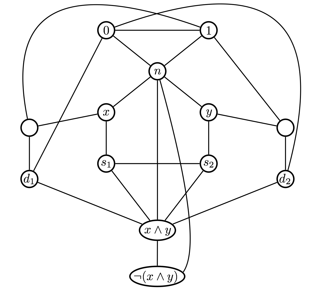
The vertices labeled with $x$ and $y$ correspond to the inputs of the NAND gate. The vertex labeled with $\neg(x\wedge y)$ corresponds to the output of the gate. We construct such a graph for each NAND gate of the circuit, however, we make sure that if, say, gate $g_1$ is an input to gate $g_2$ , then the vertex corresponding to the output of $g_1$ coincides with (is the same as) the vertex corresponding to one of the inputs of $g_2$ . Furthermore, the vertices labeled with $0$ , $1$ and $n$ are the same for each gate. In other words, in the whole graph, there is only one vertex labeled with $0$ , one vertex labeled with $1$ , and one vertex labeled with $n$ . Lastly, we put an edge between the vertex corresponding to the output vertex of the output gate and the vertex labeled with $0$ . This completes the construction of the graph $G$ . Before we prove that the reduction is correct, we make some preliminary observations.

Let’s call the $3$ colors we use to color the graph $0$ , $1$ and $n$ (we think of $n$ as “none”). Any valid coloring of $G$ must assign different colors to $3$ vertices that form a triangle (e.g. vertices labeled with $0$ , $1$ and $n$ ). If $G$ is $3$ -colorable, we can assume without loss generality that the vertex labeled $0$ is colored with the color $0$ , the vertex labeled $1$ is colored with color $1$ , and the vertex labeled $n$ is colored with the color $n$ . This is without loss of generality because if there is a valid coloring of $G$ , any permutation of the colors corresponds to a valid coloring as well. Therefore, we can permute the colors so that the labels of those vertices coincide with the colors they are colored with.

Notice that since the vertices corresponding to the inputs of a gate (i.e. the $x$ and $y$ vertices) are connected to vertex $n$ , they will be assigned the colors $0$ or $1$ . Let’s consider two cases:

If $x$ and $y$ are assigned the same color (i.e. either they are both $0$ or they are both $1$ ), the vertex labeled with $x \wedge y$ will have to be colored with that same color. That is, the vertex labeled with $x \wedge y$ must get the color corresponding to the evaluation of $x \wedge y$ . To see this, just notice that the vertices labeled $s_1$ and $s_2$ must be colored with the two colors that $x$ and $y$ are not colored with. This forces the vertex $x \wedge y$ to be colored with the same color as $x$ and $y$ .
If $x$ and $y$ are assigned different colors (i.e. one is colored with $0$ and the other with $1$ ), the vertex labeled with $x \wedge y$ will have to be colored with $0$ . That is, as in the first case, the vertex labeled with $x \wedge y$ must get the color corresponding to the evaluation of $x \wedge y$ . To see this, just notice that one of the vertices labeled $d_1$ or $d_2$ must be colored with $1$ . This forces the vertex $x \wedge y$ to be colored with $0$ since it is already connected to vertex $n$ .

In either case, the color of the vertex $x \wedge y$ must correspond to the evaluation of $x \wedge y$ . It is then easy to see that the color of the vertex $\neg (x \wedge y)$ must correspond to the evaluation of $\neg (x \wedge y)$ .

We are now ready to argue that circuit $C$ is satisfiable if and only if $G$ is $3$ -colorable. Let’s first assume that the circuit we have is satisfiable. We want to show that the graph $G$ we constructed is $3$ -colorable. Since the circuit is satisfiable, there is a 0/1 assignment to the input variables that makes the circuit evaluate to $1$ . We claim that we can use this 0/1 assignment to validly color the vertices of $G$ . We start by coloring each vertex that corresponds to an input variable: In the satisfying truth assignment, if an input variable is set to $0$ , we color the corresponding vertex with the color $0$ , and if an input variable is set to $1$ , we color the corresponding vertex with the color $1$ . As we have argued earlier, a vertex that corresponds to the output of a gate (the vertex at the very bottom of the picture above) is forced to be colored with the color that corresponds to the value that the gate outputs. It is easy to see that the other vertices, i.e., the ones labeled $s_1,s_2,d_1,d_2$ and the unlabeled vertices can be assigned valid colors. Once we color the vertices in this manner, the vertices corresponding to the inputs and output of a gate will be consistently colored with the values that it takes as input and the value it outputs. Recall that in the construction of $G$ , we connected the output vertex of the output gate with the vertex labeled with $0$ , which forces it to be assigned the color $1$ . We know this will indeed happen since the 0/1 assignment we started with makes the circuit output $1$ . This shows that we can obtain a valid $3$ -coloring of the graph $G$ .

The other direction is very similar. Assume that the constructed graph $G$ has a valid $3$ -coloring. As we have argued before, we can assume without loss of generality that the vertices labeled $0$ , $1$ , and $n$ are assigned the colors $0$ , $1$ , and $n$ respectively. We know that the vertices corresponding to the inputs of a gate must be assigned the colors $0$ or $1$ (since they are connected to the vertex labeled $n$ ). Again, as argued before, given the colors of the input vertices of a gate, the output vertex of the gate is forced to be colored with the value that the gate would output in the circuit. The fact that we can $3$ -color the graph means that the output vertex of the output gate is colored with $1$ (since it is connected to vertex $0$ and vertex $n$ by construction). This implies that the colors of the vertices corresponding to the input variables form a 0/1 assignment that makes the circuit output a $1$ , i.e. the circuit is satisfiable.

To finish the proof, we must argue that the construction of graph $G$ , given circuit $C$ , can be done in polynomial time. This is easy to see since for each gate of the circuit, we create at most a constant number of vertices and a constant number of edges. So if the circuit has $s$ gates, the construction can be done in $O(s)$ steps.

Exercise (Transitivity of Karp reductions)

Show that if $A \leq_m^PB$ and $B \leq_m^PC$ , then $A \leq_m^PC$ .

Solution

Suppose $A \leq_m^PB$ and $B \leq_m^PC$ . Let $f : \Sigma^* \to \Sigma^*$ be the map that establishes $A \leq_m^PB$ and let $g: \Sigma^* \to \Sigma^*$ be the map that establishes $B \leq_m^PC$ . So $x \in A$ if and only if $f(x) \in B$ . And $x \in B$ if and only if $g(x) \in C$ . Both $f$ and $g$ are computable in polynomial time.

To show $A \leq_m^PC$ , we define $h:\Sigma^* \to \Sigma^*$ such that $h = g \circ f$ . That is, for all $x \in \Sigma^*$ , $h(x) = g(f(x))$ . We need to show that

$x \in A$ if and only if $h(x) \in C$ ;
$h$ is computable in polynomial time.

For the first part, note that by the properties of $f$ and $g$ , $x \in A$ if and only if $f(x) \in B$ if and only if $g(f(x)) \in C$ (i.e., $h(x) \in C$ ).
(If you are having trouble following this, you can break this part up into two parts:
(i) $x\in A \implies h(x) \in C$ , (ii) $x \not \in A \implies h(x) \not \in C$ .)
For the second part, if $f$ is computable in time $O(n^k)$ , $k \geq 1$ , and $g$ is computable in time $O(n^t)$ , $t \geq 1$ , then $h$ can be computed in time $O(n^{kt})$ . (Why?)

3 Hardness and Completeness

Definition (

\mathcal{C}

-hard,

\mathcal{C}

-complete)

Let $\mathcal{C}$ be a set of languages containing $\mathsf{P}$ .

We say that $L$ is $\mathcal{C}$ -hard (with respect to Cook reductions) if for all languages $K \in \mathcal{C}$ , $K \leq^PL$ .
(With respect to polynomial time decidability, a $\mathcal{C}$ -hard language is at least as “hard” as any language in $\mathcal{C}$ .)
We say that $L$ is $\mathcal{C}$ -complete if $L$ is $\mathcal{C}$ -hard and $L \in \mathcal{C}$ .
(A $\mathcal{C}$ -complete language represents the “hardest” language in $\mathcal{C}$ with respect to polynomial time decidability.)

Note (

\mathcal{C}

-completeness and

\mathsf{P}

)

Suppose $L$ is $\mathcal{C}$ -complete. Then observe that $L \in \mathsf{P}\Longleftrightarrow \mathcal{C}= \mathsf{P}$ .

Note (

\mathcal{C}

-hardness with respect to Cook and Karp reductions)

Above we have defined $\mathcal{C}$ -hardness using Cook reductions. In literature, however, they are often defined using Karp reductions, which actually leads to a different notion of $\mathcal{C}$ -hardness. There are good reasons to use this restricted form of reductions. More advanced courses may explore some of these reasons.

4 Check Your Understanding

Problem

What is a Cook reduction? What is a Karp reduction? What is the difference between the two?
Explain why every Karp reduction can be viewed as a Cook reduction.
Explain why every Cook reduction cannot be viewed as a Karp reduction.
True or false: $\Sigma^* \leq_m^P\varnothing$ .
True or false: For languages $A$ and $B$ , $A \leq_m^PB$ if and only if $B \leq_m^PA$ .
Define the complexity class $\mathsf{P}$ .
True or false: The language $\text{251CLIQUE} = \{\langle G \rangle : \text{ $G$ is a graph containing a clique of size 251}\}$ is in $\mathsf{P}$ .
True or false: Let $L, K \subseteq \Sigma^*$ be two languages. Suppose there is a polynomial-time computable function $f : \Sigma^*\to\Sigma^*$ such that $x\in L$ iff $f(x)\notin K$ . Then $L$ Cook-reduces to $K$ .
True or false: There is a Cook reduction from 3SAT to HALTS.
For a complexity class $\mathcal{C}$ containing $\mathsf{P}$ , define what it means to be $\mathcal{C}$ -hard.
For a complexity class $\mathcal{C}$ containing $\mathsf{P}$ , define what it means to be $\mathcal{C}$ -complete.
Suppose $L$ is $\mathcal{C}$ -complete. Then argue why $L \in \mathsf{P}\Longleftrightarrow \mathcal{C}= \mathsf{P}$ .

5 High-Order Bits

Important Note

There are two very important notions of reductions introduced in this chapter: Cook reductions and Karp reductions. Make sure you understand the similarities and differences between them. And make sure you are comfortable presenting and proving the correctness of reductions. This is the main goal of the chapter.
The chapter concludes with a couple of important definitions: $\mathcal{C}$ -hardness, $\mathcal{C}$ -completeness. We present these definitions in this chapter as they are closely related to reductions. However, we will make use of these definitions in the next chapter after we introduce the complexity class $\mathsf{NP}$ . For now, make sure you understand the definitions and also Note ( $\mathcal{C}$ -completeness and $\mathsf{P}$ ).

Filters

Statement

Definition

Note

Question

Clear

Actions

Expand all

Collapse all

See overview Overview

Get PDF PDF

Give feedback Feedback

Overview: Polynomial-Time Reductions

We welcome all feedback!