
In this chapter we will briefly review the concept of mathematical induction. We assume that you are already familiar with this topic and that you have written induction proofs before. Our goal here will be to remind ourselves of the basic principle behind induction and show examples of different ways of packaging an induction argument. My hope is that this will help you understand how an induction argument works more deeply and go beyond just knowing about an induction proof template.
Hopefully you have heard about some version of the domino principle that all induction arguments are built on.
If you line up any number of dominoes in a row, and knock the first one over, then all the dominoes will fall.
The implicit assumption here is that if a domino falls, then it knocks down the next one in the row. We take this assumption as true.
The Domino Principle, as stated above, may suggest we have a finite number of dominoes. But in fact, the principle applies to infinitely many dominoes as well and this is crucial for the induction arguments we want to make. So let’s revise the domino principle and make it a statement about an infinite row of dominoes.
If you line up an infinite row of dominoes, one domino for each natural number, and you knock the first one over, then all the dominoes will fall.
When dealing with infinity, you always have to be extra careful. It is one of the trickiest concepts in mathematics, and it has tripped up many professional mathematicians in history. One of the common mistakes that beginners make is to treat infinity like any old number. But this is incorrect.
Lucky for us, even though the domino principle talks about an infinite number of dominoes, you can actually verify it using a finitary argument by employing a proof by contradiction. Let’s see how that goes.
We prove the Domino Principle by contradiction, so suppose that all the dominoes do not fall. Let domino number \(k\) be the smallest indexed domino that is standing. We know the \(k\)’th domino is not the first domino since the first one is knocked down. And since \(k\) is the smallest indexed domino that is standing, we know domino number \(k-1\) has fallen. But if domino \(k-1\) has fallen, it knocks down domino \(k\), which contradicts the assumption that domino \(k\) is standing.
As you know, in mathematical induction, the dominoes represent mathematical statements that are indexed with numbers. So suppose you want to prove that for all \(n \in \mathbb N\), \(S_n\) is true, where \(S_n\) is some mathematical statement. We can prove this if we can do the following. Let \(F_k\) correspond to “\(S_k\) is true”. First establish \(F_0\). Then show that for every \(k \in \mathbb N\), \(F_k\) implies \(F_{k+1}\). With these in hand, we can conclude that \(S_n\) is true for all \(n \in \mathbb N\). And the correctness of this follows from the way we argued that the Domino Principle is correct.
\[\begin{aligned} \textbf{Establish: } & ~~~~ \text{1. } F_0 & ~~~~ \text{(base case)} \\ & ~~~~ \text{2. for all $k$, } F_k \implies F_{k+1} & ~~~~ \text{(induction step)} \\ \textbf{Conclude: } & ~~~~ F_k \text{ for all $k$} &\end{aligned}\]
Note that there is of course flexibility in the way \(S_n\) are indexed. For instance, we may be interested in proving \(S_n\) is true for all naturals \(n \geq 251\). In this case we prove \(S_{251}\) as our base case and then show \(S_k\) implies \(S_{k+1}\) for all \(k \geq 251\). As another example, we may want to prove \(S_n\) is true for all even natural numbers. In this case we would prove \(S_0\) in our base case (assuming you define \(0\) to be a natural number) and then establish \(S_{2k}\) implies \(S_{2(k+1)}\) for naturals \(k\).
You have probably heard about strong induction as well. We prefer to refer to the previous argument as “weak induction” and refer to what is known as strong induction as just induction. Of course what you call it is not really important. The important thing is that the previous induction argument can be (and should be) strengthened. Weak induction argument asks you to establish that for all \(k \in \mathbb N\), \(F_k\) implies \(F_{k+1}\), which means you need to derive \(F_{k+1}\) assuming \(F_k\) is true. However, at this point, you can assume that \(F_0, F_1, \ldots, F_k\) are all true in order to show \(F_{k+1}\) is true. On the way to establishing \(F_k\) is true, we have established that all the lower indexed ones are true.
\[\begin{aligned} \textbf{Establish: } & ~~~~ \text{1. } F_0 & ~~~~ \text{(base case)} \\ & ~~~~ \text{2. for all $k$, } F_0, F_1, \ldots, F_k \implies F_{k+1} & ~~~~ \text{(induction step)} \\ \textbf{Conclude: } & ~~~~ F_k \text{ for all $k$} &\end{aligned}\]
Sometimes to establish \(F_{k+1}\), all you need to assume is \(F_k\). But in many scenarios, the ability to assume \(F_0, F_1, \ldots, F_k\) can be crucial to showing \(F_{k+1}\). So you might as well always assume \(F_0, F_1, \ldots, F_k\) in your induction step.
Even though you may feel that you understand induction proofs really well, my experience is that many students tend to struggle with it when the induction argument is packaged in a slightly different way than what they are used to. In particular, sometimes the \(F_k\)’s are not explicitly defined for you, sometimes \(F_k\) is a statement about a collection of objects rather than one object, and sometimes the step of establishing \(F_0, F_1, \ldots, F_k \implies F_{k+1}\) is unintuitive because it does not follow the standard weak induction template of “Assume \(F_k\), and then since x, y, z, we can conclude \(F_{k+1}\).” These and other variations can make induction proofs harder to grasp for beginners. Seeing and getting comfortable with different examples helps a lot.
So now, let’s go over some of the different ways that an induction argument can be packaged. We’ll start with the method of minimum counter-example, which we have already talked about when arguing the correctness of the Domino Principle.
We’ll first do an example, and then outline the general idea of the method of minimum counter-example.
Let’s prove that every natural number greater than 1 can be factored into primes. The method of minimum counter-example is basically an induction proof done using a proof by contradiction.
Every natural number greater than \(1\) can be factored into primes.
The proof is by contradiction, so assume the statement is false, and let \(m > 1\) be the smallest number that cannot be factored into primes. We know \(m\) is a composite number (i.e. a non-prime), so by definition, \(m = ab\), where \(1 < a,b < m\). If \(a\) and \(b\) have prime factorizations, then this would imply that \(m\) has a prime factorization. Therefore, either \(a\) or \(b\) does not have a prime factorization. But this contradicts our assumption that \(m\) is the smallest number that cannot be factored into primes.
As you can see in the proof, the way we reach the contradiction is that we chose \(m\) to be the smallest counter-example and then deduce that there is a smaller counter-example than \(m\) (either \(a\) or \(b\)). This contradicts the minimality of \(m\). Another way to think about the argument above is as follows. Let \(m\) be a counter-example (not necessarily the smallest one). Then you can continuously find smaller and smaller counter-examples. However, this is not possible since when we reach the base case (\(n=2\)), we know the statement is true.
Let’s pause here and try to really explicitly see why this is an induction argument even though the write-up of the proof does not immediately suggest so. Let \(S_n\) be the statement “\(n\) can be factored into primes”. We are trying to establish that for all \(k \geq 3\), we have \(S_2,S_3,\ldots, S_{k-1}\) implies \(S_k\). We prove this by contradiction, so we assume it is not true, which implies that there is some value of \(k\) for which \(S_2,S_3,\ldots, S_{k-1}\) does not imply \(S_k\). We let \(m\) be the minimum such number. This means we can assume \(S_2,S_3,\ldots, S_{m-1}\) are all true, but \(S_m\) is not. We then proceed to show that one of \(S_2, S_3, \ldots, S_{m-1}\) is not true and reach the desired contradiction.
Set up a proof by contradiction.
Let \(m\) be the minimum number such that \(S_m\) is not true.
Show that \(S_k\) is not true for \(k < m\), which is the desired contradiction.
Let’s now move on to invariant induction. Once again, we’ll start with an example and then outline the general strategy.
At any party, at any point in time, define a person’s parity as odd or even according to the number of hands they have shaken. Then the number of people with odd parity must be even.
Here we are not assuming anything about the number of people in total, so the statement should hold for all numbers of people. But we will not be actually inducting on the number of people.
Initially, \(0\) hands have been shaken, so \(0\) people have odd parity, i.e. and even number of people have odd parity. We now argue that this property stays invariant no matter how many handshakes occur. Consider an arbitrary point in the party and let \(t\) be the number of people with odd parity. We analyze how \(t\) changes when a handshake occurs. There are \(3\) possibilities:
Two people with odd parity shake hands. These people will no longer have odd parity, so \(t\) will go down by \(2\).
Two people with even parity shake hands. These people will no longer have even parity, so \(t\) will go up by \(2\).
A person with an odd parity shakes the hand of a person with even parity. In this case, the even parity person becomes odd parity, and the odd parity person becomes even parity. As a result, the value of \(t\) does not change.
Note that in all cases, the parity of \(t\) remains unchanged. So we can conclude that there is always an even number of people with odd parity.
So the summary is that we confirm that initially the statement is true and that with every handshake, the statement continues to be true, so we are done.
Ok, why was this an induction argument? Well, implicitly \(S_n\) is defined to be the statement that “after \(n\) handshakes, the number of people with odd parity is even.” We then proceed to show that \(S_0\) is true, and also that \(S_n\) implies \(S_{n+1}\) for all \(n\).
We have a time-varying world state: \(W_0, W_1, W_2, \ldots\).
The goal is to prove that some statement \(S\) is true for all world states.
Argue:
Statement \(S\) is true for \(W_0\).
If \(S\) is true for \(W_k\), then it remains true for \(W_{k+1}\).
So far so good. We now arrive at the final example that we will cover: structural induction. Simply put, structural induction is an induction argument proving statements about objects that can be recursively defined. Lists, strings and graphs are good examples of objects that can be defined recursively. For instance, if \(s\) a non-empty list, then \(s\) with the first element removed is also a list. Strings are similar since they can be viewed as a list of characters/symbols. More explicitly, we can define strings recursively as shown below.
Fix some finite set of symbols \(\Sigma\). We define a string over \(\Sigma\) recursively as follows.
Base case: The empty sequence, denoted \(\epsilon\), is a string.
Recursive rule: If \(x\) is a string and \(a \in \Sigma\), then \(ax\) is a string.
Note that any string (over \(\Sigma\)) can be obtained by starting from the base case and then applying the recursive rule a finite number of times.
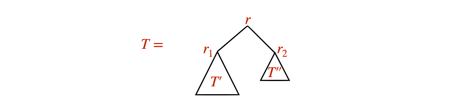
This way of defining a string hopefully gives a strong suggestion that induction can be a useful strategy in proving results about strings. Let’s make the connection explicit using another example: (rooted) binary trees. Binary trees have the following recursive structure: if you have a binary tree \(T\) with root \(r\), then the left subtree \(T'\) and the right subtree \(T''\) both are binary trees themselves.
We define a binary tree recursively as follows.
Base case: A single node \(r\) is a binary tree with root \(r\).
Recursive rule: If \(T'\) and \(T''\) are binary trees with roots \(r_1\) and \(r_2\), then \(T\), which has a node \(r\) adjacent to \(r_1\) and \(r_2\) is a binary tree with root \(r\).
Once again, any binary tree can be obtained by starting from the base case and then applying the recursive rules a finite number of times.
It turns out, in a rooted binary tree, every node has \(0\) or \(2\) children. A node with no children is called a leaf, and a node with 2 children is called an internal node.
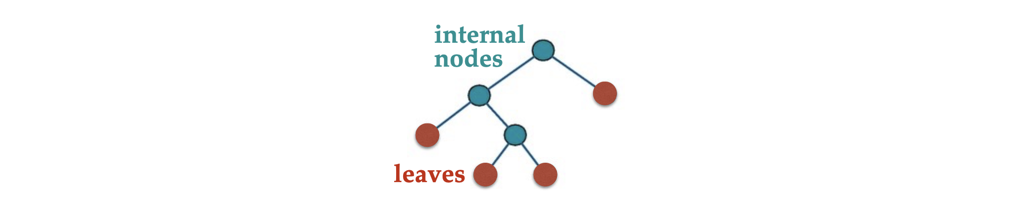
What we will now prove is that in any binary tree, the number of leaves is always exactly one more than the number of internal nodes. We will do so using an induction argument that is commonly known as structural induction. We present the proof next, and then we’ll discuss why it is a valid induction proof.
Let \(T\) be a binary tree. Let \(L_T\) be the number of leaves in \(T\) and let \(I_T\) be the number of internal nodes in \(T\). Then \(L_T = I_T + 1\).
The proof is by structural induction. In the base case \(T\) is a single node, and in this case \(L_T = 1\) and \(I_T = 0\) as desired.
To carry out the induction step, consider an arbitrary binary tree \(T\) not corresponding to the base case. Let \(T'\) be the left binary subtree of \(T\) and let \(T''\) be the right binary subtree. We know that: \[\begin{aligned} L_T & = L_{T'} + L_{T''}, & (*)\\ I_T & = I_{T'} + I_{T''} + 1. & (**)\end{aligned}\] By induction hypothesis we can assume \(L_{T'} = I_{T'} + 1\) and \(L_{T''} = I_{T''} + 1\). Our goal is to show \(L_T = I_T + 1\), and we can do so by the following chain of equalities: \[L_T \stackrel{(*)}{=} L_{T'} + L_{T''} = I_{T'} + 1 + I_{T''} + 1 \stackrel{(**)}{=} I_T + 1.\]
It is completely normal if this feels like a strange induction argument. It might very well be that it is unlike any other induction argument you have seen before.
Let’s try to dissect it a bit. First, what is the parameter \(n\) we are inducting on, and what does \(S_n\) correspond to in this particular case? The proof says “By induction hypothesis” but what is actually the induction hypothesis? Think about these questions and see if you can find satisfactory answers.
To clarify things a bit more, let’s see the general idea behind a structural induction argument.
You have a recursively defined set of objects, and you want to prove a statement \(S\) about those objects.
Check that \(S\) is true for the base case(s) of the recursive definition.
Prove \(S\) holds for “new” objects created by the recursive rule, assuming it holds for “old” objects used in the recursive rule.
In the previous example, we first confirmed the statement for the base case of a tree with a single node. We then considered an arbitrary binary tree \(T\) (not corresponding to the base case), which we think of as the “new” object created by the recursive rule. By considering the last application of the recursive rule that created \(T\), we identify \(T'\) and \(T''\) as the left and the right subtrees of \(T\), and these correspond to the “old” objects. In structural induction argument, we assume that the statement we want to prove about \(T\) already holds for the smaller/older objects \(T\) and \(T''\). And from there, with some calculations, we show that it must also hold for \(T\), completing the induction step, and the proof.
Ok, so why is this valid? Going back to the previous questions, what is the parameter we are inducting on here? What is \(S_n\)? Not just in the binary tree example we did, but in the general framework outlined above.
Let’s define \(S_n\) explicitly in the general case.
Suppose you have a set of objects \(\mathcal{O}\) defined recursively (e.g. set of rooted binary trees). And you want to show that every object in the set has some property \(P\). Define the degree of an object as the minimum number of applications of the recursive rule needed to create the object. Then we can define \(\mathcal{O}_n\) to be the set of all objects in \(\mathcal{O}\) with degree \(n\). Therefore, \(\mathcal{O}\) is the union of all the \(\mathcal{O}_n\)’s. We define \(S_n\) as the statement “every object in \(\mathcal{O}_n\) has property \(P\)”. So showing that all objects in \(\mathcal{O}\) has property \(P\) is equivalent to showing \(S_n\) for all \(n\). And when you do that using induction on \(n\), we call it structural induction.
One has to be careful with this kind of induction because often, \(S_n\) is a statement about a collection of objects, not just one. And when you want to establish, in the induction step, that \(S_0,S_1,\ldots, S_{k-1}\) implies \(S_{k}\), you need to make sure that every object in \(\mathcal{O}_k\) is covered. Let’s see an example where a mistake is made along these lines. We’ll again consider rooted binary trees.
We prove statement \(S\) by induction on the height of a tree. Let’s first check the base case... and it is true.
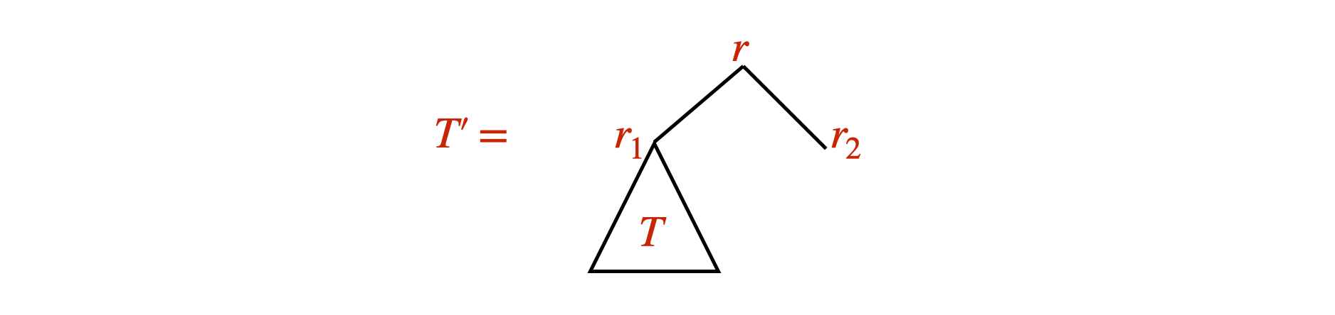
For the induction step, take an arbitrary binary tree \(T\) of height \(h\). Let \(T'\) be the following tree of height \(h+1\):
[Some argument showing why \(S\) is true for \(T'\)] Therefore we are done.
Try to articulate what is wrong with the above argument.
When we induct on height, we group the binary trees slightly differently. In particular, instead of grouping them by the number of recursive rules needed to create a binary tree, we group them according to height so that \(\mathcal{O}_n\) corresponds to all rooted binary trees of height \(n\). This strategy is perfectly fine and the correct proof we had before applies to this scenario as well. The strategy used above, however, is different. It tries to prove \(S_h\) implies \(S_{h+1}\), where \(S_h\) is “in all rooted binary trees of height \(h\), the number of leaves is one more than the number of internal nodes”. But it falls short of establishing this. It does not correctly derive \(S_{h+1}\) because it does not establish the property holds for all trees of height \(h+1\). It only establishes it for trees where the right subtree is a single node.
Let’s think more about the correct argument we presented earlier. It was kind of weird because it seemed like we were doing the induction step backwards. Let’s use height as our induction parameter. We started by considering a binary tree of some height \(h\), and then extracted the left and right subtrees that have smaller heights. Isn’t that going backwards? Shouldn’t we start with a tree of height \(h\) and then construct a tree of height \(h+1\)?
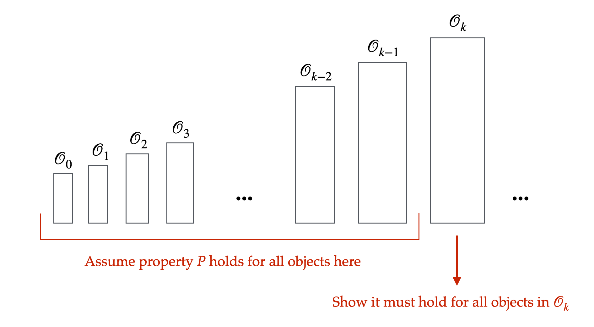
Here is a simple picture of what we want to establish in the induction step. Assuming the property holds for all objects in \(\mathcal{O}_0, \mathcal{O}_1, \ldots, \mathcal{O}_{k-1}\), we want to show that it holds for all objects in \(\mathcal{O}_k\). We have to make sure that in our argument we cover all the objects in \(\mathcal{O}_k\). We can’t leave anything out. With that in mind, we start the argument as “Consider an arbitrary object \(T\) of \(\mathcal{O}_k\)” with the intention of showing that \(T\) has property \(P\). Note that if we are able to do this, then we are done! Because when you show something is true for an arbitrary object in a set, you show it for all the objects in the set.
Also notice that we want to show \(\mathcal{O}_0, \mathcal{O}_1, \ldots, \mathcal{O}_{k-1}\) implies \(\mathcal{O}_k\) for all \(k\). So we might as well consider an arbitrary \(k > 0\). It shouldn’t matter what it is. This is why in our argument, we actually started with “Consider an arbitrary object \(T\)” without any reference to a parameter \(k\).
Great, so we start with “Consider an arbitrary tree \(T\) (not corresponding to the base case)”. It implicitly belongs to \(\mathcal{O}_k\) for some \(k > 0\). Then what do we do? Well, \(T\) has a recursive structure, so we view it as being composed of one or more “smaller” objects in \(\mathcal{O}_0, \mathcal{O}_1, \ldots, \mathcal{O}_{k-1}\). The power of induction gives us the ability to assume that these smaller objects do have property \(P\). Using this, we proceed to show that \(T\) must also have property \(P\). And we are done.
As you can see, we were never going backwards in our induction step and that we were indeed arguing \(S_0, S_1, \ldots, S_{k-1}\) implies \(S_k\).
We will leave you with one last example/exercise. This one involves a set of binary strings that is defined recursively. Please attempt to prove it yourself using structural induction. This is very important. If you are able to do it, that is awesome! If not, hopefully you will be able to identify where your understanding might be lacking. And that is very valuable. You can go back and try to fill in the gaps yourself, or let us know, and we would be happy to help out.
Let \(L\) be a set of binary strings (i.e. strings over \(\Sigma = \{{\texttt{0}}, {\texttt{1}}\}\)) defined recursively as follows:
(base case) the empty string, \(\epsilon\), is in \(L\);
(recursive rule) if \(x, y \in L\), then \({\texttt{0}}x{\texttt{1}}y{\texttt{0}} \in L\).
This means that every string in \(L\) is derived starting from the base case, and applying the recursive rule a finite number of times. Show that for any string \(w \in L\), the number of \({\texttt{0}}\)’s in \(w\) is exactly twice the number of \({\texttt{1}}\)’s in \(w\).
Let \(\mathbf{0}(w)\) denote the number of \({\texttt{0}}\)’s in \(w\) and let \(\mathbf{1}(w)\) denote the number of \({\texttt{1}}\)’s in \(w\). Given \(L\) as defined above, the question asks us to show that for any \(w \in L\), \(\mathbf{0}(w) = 2 \cdot \mathbf{1}(w)\). We will do so by structural induction.
The base case corresponds to \(w = \epsilon\), and in this case, \(\mathbf{0}(w) = \mathbf{1}(w) = 0\), and therefore \(\mathbf{0}(w) = 2 \cdot \mathbf{1}(w)\) holds.
To carry out the induction step, consider an arbitrary string \(w \neq \epsilon\) in \(L\). Then by the definition of \(L\), we know that there exists \(x\) and \(y\) in \(L\) such that \(w = {\texttt{0}}x{\texttt{1}}y{\texttt{0}}\). Furthermore, by induction hypothesis, \[\mathbf{0}(x) = 2 \cdot \mathbf{1}(x) \quad \quad (*)\] and \[\mathbf{0}(y) = 2 \cdot \mathbf{1}(y). \quad \quad (**)\] We are done once we show \(\mathbf{0}(w) = 2 \cdot \mathbf{1}(w)\). We establish this via the following chain of equalities: \[\begin{aligned} \mathbf{0}(w) & = 2 + \mathbf{0}(x) + \mathbf{0}(y) & \text{since $w = {\texttt{0}}x{\texttt{1}}y{\texttt{0}}$} \\ & = 2 + 2 \cdot \mathbf{1}(x) + 2 \cdot \mathbf{1}(y) & \text{by $(*)$ and $(**)$}\\ & = 2 \cdot (1 + \mathbf{1}(x) + \mathbf{1}(y)) \\ & = 2 \cdot \mathbf{1}(w).\end{aligned}\]
In an induction argument on recursively defined objects, if you say that you will use structural induction, then the assumption is that the parameter being inducted on is the minimum number of applications of the recursive rules needed to create an object. And in this case, explicitly stating the parameter being inducted on, or the induction hypothesis, is not needed.
As a final remark, we want to emphasize that even though we gave different names to the induction proofs we have seen in this chapter, they are really all the same kind of argument. They all follow the basic (strong) induction proof strategy. So this was not about teaching you new proof strategies, not at all, but rather about seeing examples of how a regular induction proof can manifest itself in different settings. And hopefully, this has made you appreciate and understand induction proofs better.
This marks the end of this chapter. If you have any questions about anything, don’t hesitate to ask!