In this chapter, our main goal is to introduce the definition of a Turing machine, which is the standard mathematical model for any kind of computational device. As such, this definition is very foundational. As we discuss in lecture, the physical Church-Turing thesis asserts that any kind of physical device or phenomenon, when viewed as a computational process mapping input data to output data, can be simulated by some Turing machine. Thus, rigorously studying Turing machines does not just give us insights about what our laptops can or cannot do, but also tells us what the universe can and cannot do computationally.
This chapter kicks things off with examples of decidable languages (i.e. decision problems that we can compute). Later, we will start exploring the limitations of computation. Some of the examples we cover in this chapter will serve as a warm-up to other examples we will discuss in the next chapter in the context of uncomputability.
A Turing machine (TM) \(M\) is a 7-tuple \[M = (Q, \Sigma, \Gamma, \delta, q_0, q_\text{acc}, q_\text{rej}),\] where
\(Q\) is a non-empty finite set
(which we refer to as the set of states of the TM);\(\Sigma\) is a non-empty finite set that does not contain the blank symbol \(\sqcup\)
(which we refer to as the input alphabet of the TM);\(\Gamma\) is a finite set such that \(\sqcup\in \Gamma\) and \(\Sigma \subset \Gamma\)
(which we refer to as the tape alphabet of the TM);\(\delta\) is a function of the form \(\delta: Q \times \Gamma \to Q \times \Gamma \times \{\text{L}, \text{R}\}\)
(which we refer to as the transition function of the TM);\(q_0 \in Q\) is an element of \(Q\)
(which we refer to as the initial state of the TM or the starting state of the TM);\(q_\text{acc}\in Q\) is an element of \(Q\)
(which we refer to as the accepting state of the TM);\(q_\text{rej}\in Q\) is an element of \(Q\) such that \(q_\text{rej}\neq q_\text{acc}\)
(which we refer to as the rejecting state of the TM).
Allowing the tape alphabet to be any finite set containing the blank symbol and the input alphabet gives us flexibility when designing a TM. On the other hand, this flexibility is only for convenience and does not give extra computational power to the TM computational model.
Similar to DFAs, we’ll consider two Turing machines to be equivalent/same if they are the same machine up to renaming the elements of the sets \(Q\), \(\Sigma\) and \(\Gamma\).
In the transition function \(\delta\) of a TM, we don’t really care about how we define the output of \(\delta\) when the input state is \(q_\text{acc}\) or \(q_\text{rej}\) because once the computation reaches one of these states, it stops. We explain this below in Definition (Computation path for a TM).
Below is an example of a state diagram of a TM with \(5\) states:
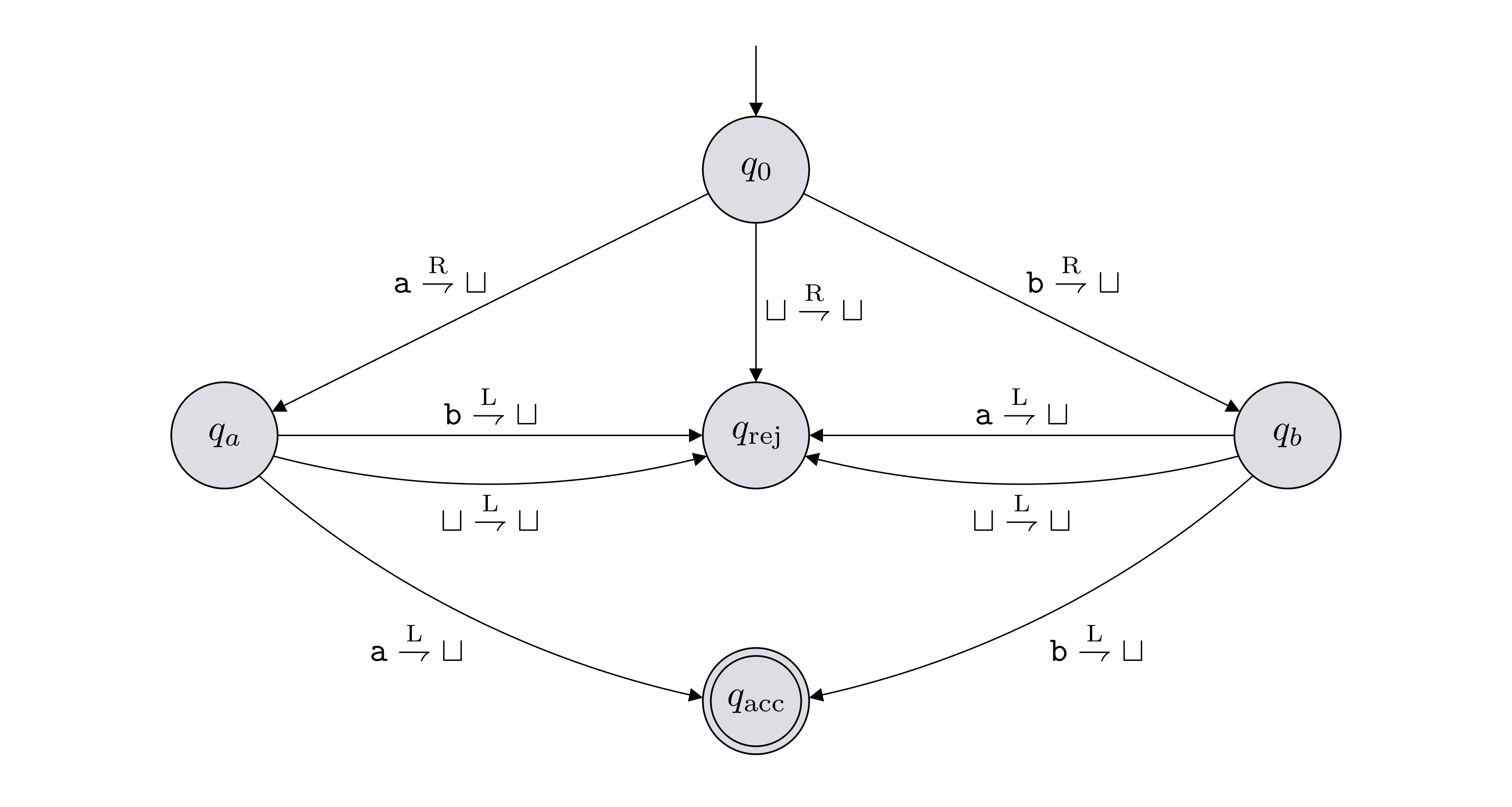
In this example, \(\Sigma = \{{\texttt{a}},{\texttt{b}}\}\), \(\Gamma = \{{\texttt{a}},{\texttt{b}},\sqcup\}\), \(Q = \{q_0,q_a,q_b,q_\text{acc},q_\text{rej}\}\). The labeled arrows between the states encode the transition function \(\delta\). As an example, the label on the arrow from \(q_0\) to \(q_a\) is \({\texttt{a}} \overset{\text{R}}{\rightharpoondown} \sqcup\), which represents \(\delta(q_0, {\texttt{a}}) = (q_a, \sqcup, \text{R})\)
A Turing machine is always accompanied by a tape that is used as memory. The tape is just a sequence of cells that can hold any symbol from the tape alphabet. The tape can be defined so that it is infinite in two directions (so we could imagine indexing the cells using the integers \(\mathbb Z\)), or it could be infinite in one direction, to the right (so we could imagine indexing the cells using the natural numbers \(\mathbb N\)). The input to a Turing machine is always a string \(w \in \Sigma^*\). The string \(w_1\ldots w_n \in \Sigma^*\) is put on the tape so that symbol \(w_i\) is placed on the cell with index \(i-1\). We imagine that there is a tape head that initially points to index 0. The symbol that the tape head points to at a particular time is the symbol that the Turing machine reads. The tape head moves left or right according to the transition function of the Turing machine. These details are explained in lecture.
In these notes, we assume our tape is infinite in two directions.
Given any DFA and any input string, the DFA always halts and makes a decision to either reject or accept the string. The same is not true for TMs and this is an important distinction between DFAs and TMs. It is possible that a TM does not make a decision when given an input string, and instead, loops forever. So given a TM \(M\) and an input string \(x\), there are 3 options when we run \(M\) on \(x\):
\(M\) accepts \(x\) (denoted \(M(x) = 1\));
\(M\) rejects \(x\) (denoted \(M(x) = 0\));
\(M\) loops forever (denoted \(M(x) = \infty\)).
The formal definitions for these 3 cases is given below.
Let \(M\) be a Turing machine where \(Q\) is the set of states, \(\sqcup\) is the blank symbol, and \(\Gamma\) is the tape alphabet. To understand how \(M\)’s computation proceeds we generally need to keep track of three things: (i) the state \(M\) is in; (ii) the contents of the tape; (iii) where the tape head is. These three things are collectively known as the “configuration” of the TM. More formally: a configuration for \(M\) is defined to be a string \(uqv \in (\Gamma \cup Q)^*\), where \(u, v \in \Gamma^*\) and \(q \in Q\). This represents that the tape has contents \(\cdots \sqcup\sqcup\sqcup uv \sqcup\sqcup\sqcup\cdots\), the head is pointing at the leftmost symbol of \(v\), and the state is \(q\). A configuration is an accepting configuration if \(q\) is \(M\)’s accept state and it is a rejecting configuration if \(q\) is \(M\)’s reject state.
Suppose that \(M\) reaches a certain configuration \(\alpha\) (which is not accepting or rejecting). Knowing just this configuration and \(M\)’s transition function \(\delta\), one can determine the configuration \(\beta\) that \(M\) will reach at the next step of the computation. (As an exercise, make this statement precise.) We write \[\alpha \vdash_M \beta\] and say that “\(\alpha\) yields \(\beta\) (in \(M\))”. If it is obvious what \(M\) we’re talking about, we drop the subscript \(M\) and just write \(\alpha \vdash \beta\).
Given an input \(x \in \Sigma^*\) we say that \(M(x)\) halts if there exists a sequence of configurations (called the computation path) \(\alpha_0, \alpha_1, \dots, \alpha_{T}\) such that:
\(\alpha_0 = q_0x\), where \(q_0\) is \(M\)’s initial state;
\(\alpha_t \vdash_M \alpha_{t+1}\) for all \(t = 0, 1, 2, \dots, T-1\);
\(\alpha_T\) is either an accepting configuration (in which case we say \(M(x)\) accepts) or a rejecting configuration (in which case we say \(M(x)\) rejects).
Otherwise, we say \(M(x)\) loops.
Let \(M\) denote the Turing machine shown below, which has input alphabet \(\Sigma = \{{\texttt{0}}\}\) and tape alphabet \(\Gamma = \{{\texttt{0}},{\texttt{x}}, \sqcup\}\).
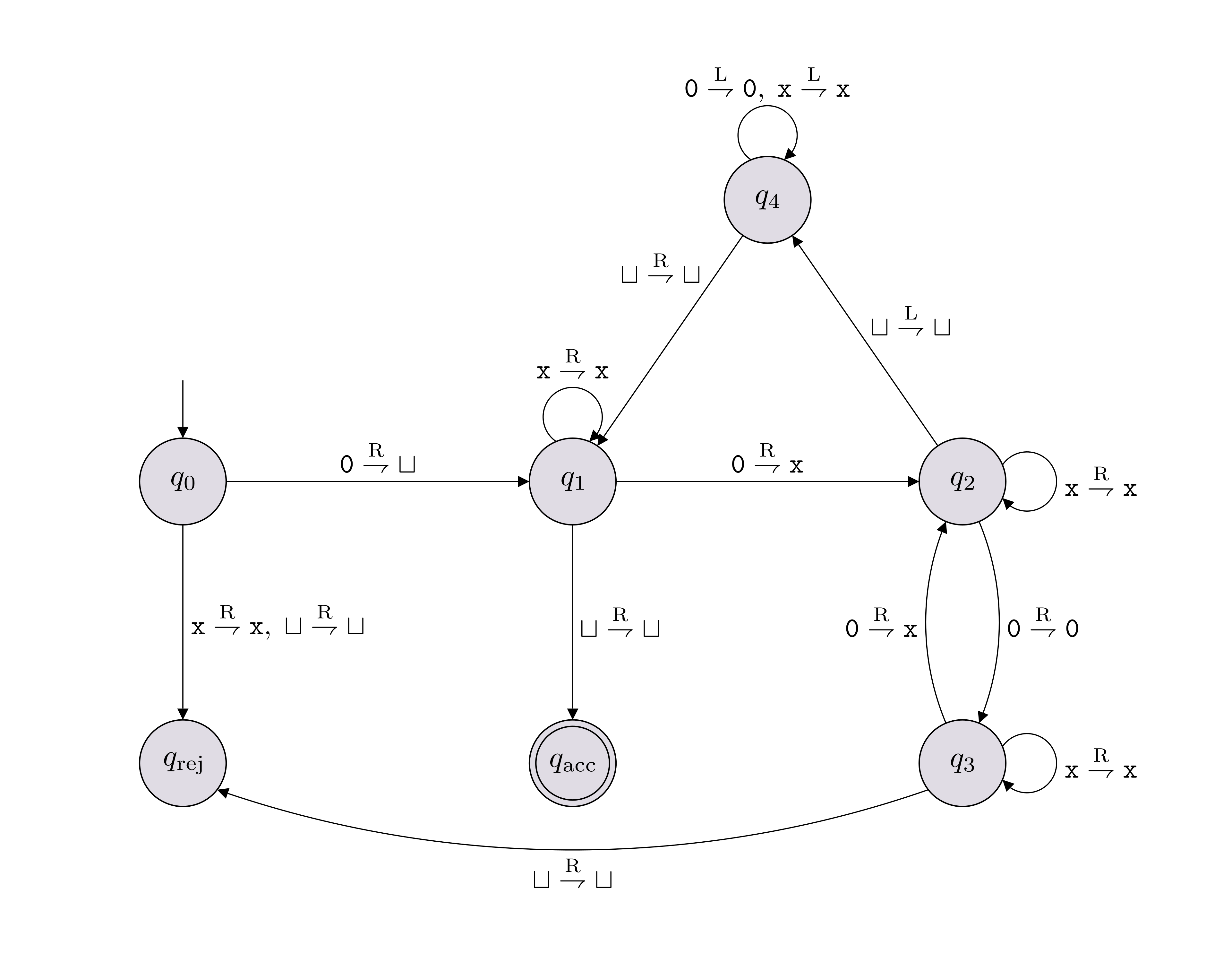
Write out the computation path \[\alpha_0 \vdash_M \alpha_1 \vdash_M \cdots \vdash_M \alpha_T\] for \(M({\texttt{0000}})\) and determine whether it accepts or rejects.
Read down first and then to the right. \[\begin{aligned} q_0{\texttt{0000}} \qquad q_4{\texttt{x0x}} \qquad & {\texttt{x}}q_4{\texttt{xx}} \\ q_1{\texttt{000}} \quad q_4\sqcup{\texttt{x0x}} \qquad & q_4{\texttt{xxx}} \\ {\texttt{x}}q_2{\texttt{00}} \qquad q_1{\texttt{x0x}} \qquad & q_4\sqcup{\texttt{xxx}} \\ {\texttt{x0}}q_3{\texttt{0}} \qquad {\texttt{x}}q_1{\texttt{0x}} \qquad & q_1{\texttt{xxx}} \\ {\texttt{x0x}}q_2 \qquad {\texttt{xx}}q_2{\texttt{x}} \qquad & {\texttt{x}}q_1{\texttt{xx}} \\ {\texttt{x0}}q_4{\texttt{x}} \qquad {\texttt{xxx}}q_2 \qquad & {\texttt{xx}}q_1{\texttt{x}} \\ {\texttt{x}}q_4{\texttt{0x}} \qquad {\texttt{xx}}q_4{\texttt{x}} \qquad & {\texttt{xxx}}q_1 \\ & {\texttt{xxx}} \sqcup q_\text{acc}\end{aligned}\] \(M({\texttt{0000}})\) accepts.
Let \(f: \Sigma^* \to \{0,1\}\) be a decision problem and let \(M\) be a TM with input alphabet \(\Sigma\). We say that \(M\) solves (or decides, or computes) \(f\) if the input/output behavior of \(M\) matches \(f\) exactly, in the following sense: for all \(w \in \Sigma^*\), \(M(w) = f(w)\).
If \(L\) is the language corresponding to \(f\), the above definition is equivalent to saying that \(M\) solves (or decides, or computes) \(L\) if the following holds:
if \(w \in L\), then \(M\) accepts \(w\) (i.e. \(M(w) = 1\));
if \(w \not \in L\), then \(M\) rejects \(w\) (i.e. \(M(w) = 0\)).
If \(M\) solves a decision problem (language), \(M\) must halt on all inputs. Such a TM is called a decider.
The language of a TM \(M\) is \[L(M) = \{w \in \Sigma^* : \text{$M$ accepts $w$}\}.\] Given a TM \(M\), we cannot say that \(M\) solves/decides \(L(M)\) because \(M\) may loop forever for inputs \(w\) not in \(L(M)\). Only a decider TM can decide a language. And if \(M\) is indeed a decider, then \(L(M)\) is the unique language that \(M\) solves/decides.
The language decided by the TM is \[L = \{w \in \{a,b\}^* : |w| \geq 2 \text{ and } w_1 = w_2\}.\]
For each language below, draw the state diagram of a TM that decides the language. You can use any finite tape alphabet \(\Gamma\) containing the elements of \(\Sigma\) and the symbol \(\sqcup\).
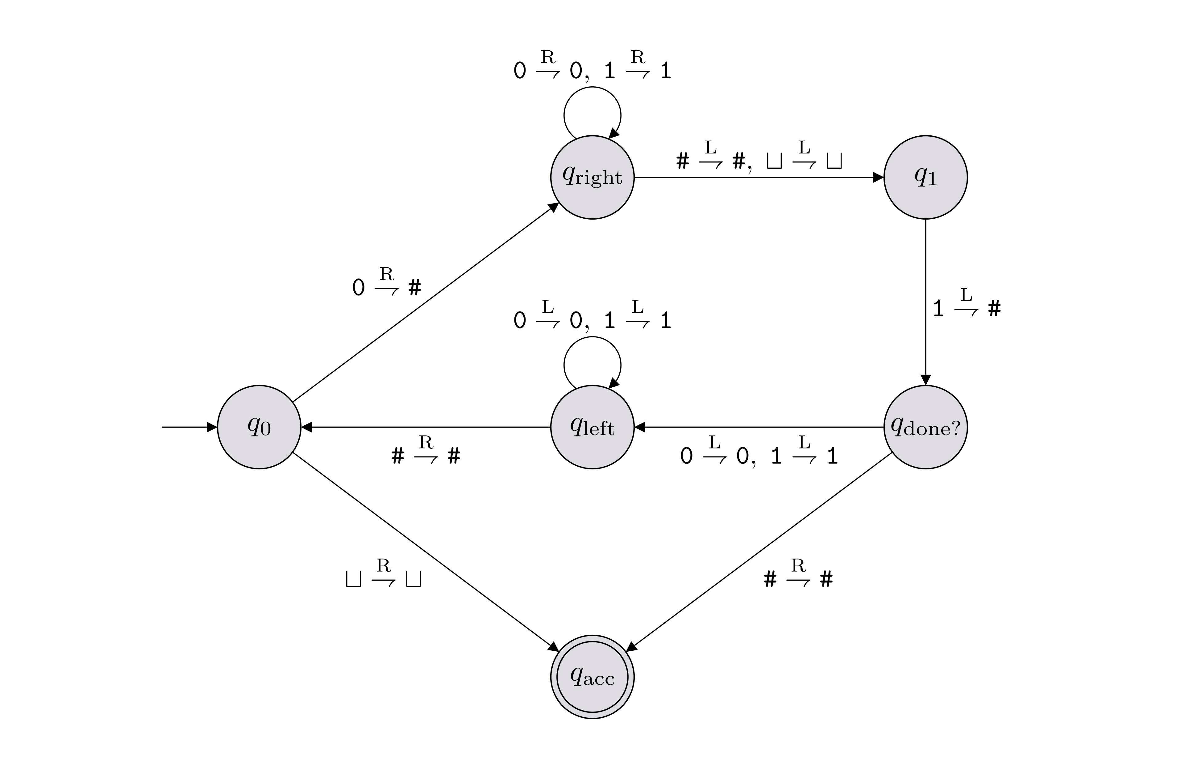
\(L = \{{\texttt{0}}^n{\texttt{1}}^n : n \in \mathbb N\}\), where \(\Sigma = \{{\texttt{0}},{\texttt{1}}\}\).
\(L = \{{\texttt{0}}^{2^n} : n \in \mathbb N\}\), where \(\Sigma = \{{\texttt{0}}\}\).
Our TM will have the tape alphabet \(\Gamma = \{{\texttt{0}},{\texttt{1}},{\texttt{\#}}, \sqcup\}\). The rejecting state is omitted from the state diagram below. All the missing transitions go to the rejecting state.
See the figure in Exercise (Practice with configurations), part 2.
A language \(L\) is called decidable (or computable) if there exists a TM that decides (i.e. solves) \(L\).
We denote by \(\mathsf{R}\) the set of all decidable languages (over the default alphabet \(\Sigma = \{{\texttt{0}}, {\texttt{1}}\}\)).
A decidable language is also called a recursive language, and \(\mathsf{R}\) is the standard notation used in the literature for representing the set of all decidable/recursive languages.
So far, with DFAs and TMs, we talked about machines solving languages (i.e. decision problems). Unlike DFAs, there is a natural way to interpret TMs as solving more general computational problems.
Let \(M\) be a TM with input alphabet \(\Sigma\). We say that on input \(x\), \(M\) outputs the string \(y\) if the following hold:
\(M(x)\) halts with the halting configuration being \(uqv\) (where \(q \in \{q_\text{acc}, q_\text{rej}\}\)),
the string \(uv\) equals \(y\).
In this case we write \(M(x) = y\).
We say \(M\) solves (or computes) a function problem \(f : \Sigma^* \to \Sigma^*\) if for all \(x \in \Sigma^*\), \(M(x) = f(x)\).
The Church-Turing Thesis (CTT) states that any computation that can be conducted in this universe (constrained by the laws of physics of course), can be carried out by a TM. In other words, the set of problems that are in principle computable in this universe is captured by the complexity class \(\mathsf{R}\).
There are a couple of important things to highlight. First, CTT says nothing about the efficiency of the simulation. Second, CTT is not a mathematical statement, but a physical claim about the universe we live in (similar to claiming that the speed of light is constant). The implications of CTT is far-reaching. For example, CTT claims that any computation that can be carried out by a human can be carried out by a TM. Other implications are discussed in lecture.
We will consider three different ways of describing TMs.
A low-level description of a TM is given by specifying the 7-tuple in its definition. This information is often presented using a picture of its state diagram.
A medium-level description is an English description of the movement and behavior of the tape head, as well as how the contents of the tape is changing, as the computation is being carried out.
A high-level description is pseudocode or an algorithm written in English. Usually, an algorithm is written in a way so that a human can read it, understand it, and carry out its steps. By CTT, there is a TM that can carry out the same computation.
Unless explicitly stated otherwise, you can present a TM using a high-level description. From now on, we will do the same.
Let’s consider the language \(L = \{{\texttt{0}}^n {\texttt{1}}^n : n \in \mathbb N\}\). The solution to Exercise (Drawing TM state diagrams) has a low-level description of a TM deciding \(L\).
Here is an example of a medium-level description of a TM deciding \(L\).
  Repeat:
    If the current symbol is a blank or #, accept.
    Else if the symbol is a 1, reject.
    Else, cross off the 0 symbol with #.
    Move to the right until a blank or # is reached.
    Move one index to the left.
    If the symbol is not a 1 reject.
    Else, cross off the 1 symbol with a #.
    Move to the left until a # symbol is reached.
    Move one index to the right.
And here is a high-level decider for \(L\). \[\begin{aligned} \hline\hline\\[-12pt] &\textbf{def}\;\; M(x):\\ &{\scriptstyle 1.}~~~~\texttt{$n = |x|$.}\\ &{\scriptstyle 2.}~~~~\texttt{If $n$ is not even, reject.}\\ &{\scriptstyle 3.}~~~~\texttt{For $i = 1, 2, \ldots, n/2$:}\\ &{\scriptstyle 4.}~~~~~~~~\texttt{If $x_i = 1$ or $x_{n-i+1} = 0$, reject.}\\ &{\scriptstyle 5.}~~~~\texttt{Accept.}\\ \hline\hline\end{aligned}\]
Let \(L\) and \(K\) be decidable languages. Show that \(\overline{L} = \Sigma^* \setminus L\), \(L \cap K\) and \(L \cup K\) are also decidable by presenting high-level descriptions of TMs deciding them.
Since \(L\) and \(K\) are decidable, there are decider TMs \(M_L\) and \(M_K\) such that \(L(M_L) = L\) and \(L(M_K) = K\).
To show \(\overline{L}\) is decidable, we present a high-level description of a TM \(M\) deciding it: \[\begin{aligned} \hline\hline\\[-12pt] &\textbf{def}\;\; M(x):\\ &{\scriptstyle 1.}~~~~\texttt{Run $M_L(x)$.}\\ &{\scriptstyle 2.}~~~~\texttt{If it accepts, reject.}\\ &{\scriptstyle 3.}~~~~\texttt{If it rejects, accept.}\\ \hline\hline\end{aligned}\]
It is pretty clear that this decider works correctly.
To show \(L \cup K\) is decidable, we present a high-level description of a TM \(M\) deciding it: \[\begin{aligned} \hline\hline\\[-12pt] &\textbf{def}\;\; M(x):\\ &{\scriptstyle 1.}~~~~\texttt{Run $M_L(x)$. If it accepts, accept.}\\ &{\scriptstyle 2.}~~~~\texttt{Run $M_K(x)$. If it accepts, accept.}\\ &{\scriptstyle 3.}~~~~\texttt{Reject.}\\ \hline\hline\end{aligned}\]
Once again, it is pretty clear that this decider works correctly. However, in case you are wondering how in general (with more complicated examples) we would prove that a decider works as desired, here is an example argument.
Following Definition (TM solving/deciding a language or decision problem), we want to show that if \(x \in L \cup K\), then \(M(x)\) accepts, and if \(x \not \in L \cup K\), then \(M(x)\) rejects. If \(x \in L \cup K\), then it is either in \(L\) or in \(K\). If it is in \(L\), then \(M_L(x)\) accepts (since \(M_L\) correctly decides \(L\)) and therefore \(M\) accepts on line 1. If, on the other hand, \(x \in K\), then \(M_K(x)\) accepts. This means that if \(M\) does not accept on line 1, then it has to accept on line 2. Either way \(x\) is accepted by \(M\). For the second part, assume \(x \not \in L \cup K\). This means \(x \not \in L\) and \(x \not \in K\). Therefore \(M(x)\) will not accept on line 1 and it will not accept on line 2. And so it rejects on line 3, as desired.
To show \(L \cap K\) is decidable, we present a high-level description of a TM \(M\) deciding it: \[\begin{aligned} \hline\hline\\[-12pt] &\textbf{def}\;\; M(x):\\ &{\scriptstyle 1.}~~~~\texttt{Run $M_L(x)$ and $M_K(x)$.}\\ &{\scriptstyle 2.}~~~~\texttt{If they both accept, accept.}\\ &{\scriptstyle 3.}~~~~\texttt{Else, reject.}\\ \hline\hline\end{aligned}\]
Fix \(\Sigma = \{{\texttt{3}}\}\) and let \(L \subseteq \{{\texttt{3}}\}^*\) be defined as follows: \(x \in L\) if and only if \(x\) appears somewhere in the decimal expansion of \(\pi\). For example, the strings \(\epsilon\), \({\texttt{3}}\), and \({\texttt{33}}\) are all definitely in \(L\), because \[\pi = 3.1415926535897932384626433\dots\] Prove that \(L\) is decidable. No knowledge in number theory is required to solve this question.
The important observation is the following. If, for some \(m \in \mathbb N\), \({\texttt{3}}^m\) is not in \(L\), then neither is \({\texttt{3}}^{k}\) for any \(k > m\). Additionally, if \({\texttt{3}}^m \in L\), then so is \({\texttt{3}}^{\ell}\) for every \(\ell < m\). For each \(n \in \mathbb N\), define \[L_n = \{{\texttt{3}}^m : m \leq n\}.\] Then either \(L = L_n\) for some \(n\), or \(L = \{{\texttt{3}}\}^*\).
If \(L = L_n\) for some \(n\), then the following TM decides it.
\[\begin{aligned} \hline\hline\\[-12pt] &\textbf{def}\;\; M(x):\\ &{\scriptstyle 1.}~~~~\texttt{If $|x| \leq n$, accept.}\\ &{\scriptstyle 2.}~~~~\texttt{Else, reject.}\\ \hline\hline\end{aligned}\]
If \(L = \{{\texttt{3}}\}^*\), then it is decided by:
\[\begin{aligned} \hline\hline\\[-12pt] &\textbf{def}\;\; M(x):\\ &{\scriptstyle 1.}~~~~\texttt{Accept.}\\ \hline\hline\end{aligned}\]
So in all cases, \(L\) is decidable.
In Chapter 1 we saw that we can use the notation \(\left \langle \cdot \right\rangle\) to denote an encoding of objects belonging to any countable set. For example, if \(D\) is a DFA, we can write \(\left \langle D \right\rangle\) to denote the encoding of \(D\) as a string. If \(M\) is a TM, we can write \(\left \langle M \right\rangle\) to denote the encoding of \(M\). There are many ways one can encode DFAs and TMs. We will not be describing a specific encoding scheme as this detail will not be important for us.
Recall that when we want to encode a tuple of objects, we use the comma sign. For example, if \(M_1\) and \(M_2\) are two Turing machines, we write \(\left \langle M_1, M_2 \right\rangle\) to denote the encoding of the tuple \((M_1,M_2)\). As another example, if \(M\) is a TM and \(x \in \Sigma^*\), we can write \(\left \langle M, x \right\rangle\) to denote the encoding of the tuple \((M,x)\).
The fact that we can encode a Turing machine (or a piece of code) means that an input to a TM can be the encoding of another TM (in fact, a TM can take the encoding of itself as the input). This point of view has several important implications, one of which is the fact that we can come up with a Turing machine, which given as input the description of any Turing machine, can simulate it. This simulator Turing machine is called a universal Turing machine.
Let \(\Sigma\) be some finite alphabet. A universal Turing machine \(U\) is a Turing machine that takes \(\left \langle M, x \right\rangle\) as input, where \(M\) is a TM and \(x\) is a word in \(\Sigma^*\), and has the following high-level description:
\[\begin{aligned} \hline\hline\\[-12pt] &\textbf{def}\;\; U(\left \langle \text{TM } M, \; \text{string } x \right\rangle):\\ &{\scriptstyle 1.}~~~~\texttt{Simulate $M$ on input $x$ (i.e. run $M(x)$)}\\ &{\scriptstyle 2.}~~~~\texttt{If it accepts, accept.}\\ &{\scriptstyle 3.}~~~~\texttt{If it rejects, reject.}\\ \hline\hline\end{aligned}\]
Note that if \(M(x)\) loops forever, then \(U\) loops forever as well. To make sure \(M\) always halts, we can add a third input, an integer \(k\), and have the universal machine simulate the input TM for at most \(k\) steps.
Above, when denoting the encoding of a tuple \((M, x)\) where \(M\) is a Turing machine and \(x\) is a string, we used \(\left \langle \text{TM } M, \text{string } x \right\rangle\) to make clear what the types of \(M\) and \(x\) are. We will make use of this notation from now on and specify the types of the objects being referenced within the encoding notation.
When we give a high-level description of a TM, we often assume that the input given is of the correct form/type. For example, with the Universal TM above, we assumed that the input was the encoding \(\left \langle \text{TM } M, \; \text{string } x \right\rangle\). But technically, the input to the universal TM (and any other TM) is allowed to be any finite-length string. What do we do if the input string does not correspond to a valid encoding of an expected type of input object?
Even though this is not explicitly written, we will implicitly assume that the first thing our machine does is check whether the input is a valid encoding of objects with the expected types. If it is not, the machine rejects. If it is, then it will carry on with the specified instructions.
The important thing to keep in mind is that in our descriptions of Turing machines, this step of checking whether the input string has the correct form (i.e. that it is a valid encoding) will never be explicitly written, and we don’t expect you to explicitly write it either. That being said, be aware that this check is implicitly there.
The languages \(\text{ACCEPTS}_{\text{DFA}}\) and \(\text{SA}_{\text{DFA}}\) are decidable.
Our goal is to show that \(\text{ACCEPTS}_{\text{DFA}}\) and \(\text{SA}_{\text{DFA}}\) are decidable languages. To show that these languages are decidable, we will give high-level descriptions of TMs deciding them.
For \(\text{ACCEPTS}_{\text{DFA}}\), the decider is essentially the same as a universal TM:
\[\begin{aligned} \hline\hline\\[-12pt] &\textbf{def}\;\; M(\left \langle \text{DFA } D, \; \text{string } x \right\rangle):\\ &{\scriptstyle 1.}~~~~\texttt{Simulate $D$ on input $x$ (i.e. run $D(x)$)}\\ &{\scriptstyle 2.}~~~~\texttt{If it accepts, accept.}\\ &{\scriptstyle 3.}~~~~\texttt{If it rejects, reject.}\\ \hline\hline\end{aligned}\]
It is clear that this correctly decides \(\text{ACCEPTS}_{\text{DFA}}\).
For \(\text{SA}_{\text{DFA}}\), we just need to slightly modify the above machine:
\[\begin{aligned} \hline\hline\\[-12pt] &\textbf{def}\;\; M(\left \langle \text{DFA } D \right\rangle):\\ &{\scriptstyle 1.}~~~~\texttt{Simulate $D$ on input $\left \langle D \right\rangle$ (i.e. run $D(\left \langle D \right\rangle)$)}\\ &{\scriptstyle 2.}~~~~\texttt{If it accepts, accept.}\\ &{\scriptstyle 3.}~~~~\texttt{If it rejects, reject.}\\ \hline\hline\end{aligned}\]
Again, it is clear that this correctly decides \(\text{SA}_{\text{DFA}}\).
The language \(\text{SAT}_{\text{DFA}}\) is decidable.
Our goal is to show \(\text{SAT}_{\text{DFA}}\) is decidable and we will do so by constructing a decider for \(\text{SAT}_{\text{DFA}}\).
A decider for \(\text{SAT}_{\text{DFA}}\) takes as input \(\left \langle D \right\rangle\) for some DFA \(D = (Q, \Sigma, \delta, q_0, F)\), and needs to determine if \(D\) is satisfiable (i.e. if there is any input string that \(D\) accepts). If we view the DFA as a directed graph, where the states of the DFA correspond to the nodes in the graph and transitions correspond to edges, notice that the DFA accepts some string if and only if there is a directed path from \(q_0\) to some state in \(F\). Therefore, the following decider decides \(\text{SAT}_{\text{DFA}}\) correctly.
\[\begin{aligned} \hline\hline\\[-12pt] &\textbf{def}\;\; M(\left \langle \text{DFA } D \right\rangle):\\ &{\scriptstyle 1.}~~~~\texttt{Build a directed graph from $\left \langle D \right\rangle$.}\\ &{\scriptstyle 2.}~~~~\texttt{Run a graph search algorithm starting from $q_0$ of $D$.}\\ &{\scriptstyle 3.}~~~~\texttt{If a node corresponding to an accepting state is reached, accept.}\\ &{\scriptstyle 4.}~~~~\texttt{Else, reject.}\\ \hline\hline\end{aligned}\]
The language \(\text{NEQ}_{\text{DFA}}\) is decidable.
Our goal is to show that \(\text{NEQ}_{\text{DFA}}\) is decidable. We will do so by constructing a decider for \(\text{NEQ}_{\text{DFA}}\).
Our argument is going to use Theorem (\(\text{SAT}_{\text{DFA}}\) is decidable). In particular, the decider we present for \(\text{NEQ}_{\text{DFA}}\) will use the decider for \(\text{SAT}_{\text{DFA}}\) as a subroutine. Let \(M\) denote a decider TM for \(\text{SAT}_{\text{DFA}}\).
A decider for \(\text{NEQ}_{\text{DFA}}\) takes as input \(\left \langle D_1,D_2 \right\rangle\), where \(D_1\) and \(D_2\) are DFAs. It needs to determine if \(L(D_1) \neq L(D_2)\) (i.e. accept if \(L(D_1) \neq L(D_2)\) and reject otherwise). We can determine if \(L(D_1) \neq L(D_2)\) by looking at their symmetric difference of \(L(D_1)\) and \(L(D_2)\): \[(L(D_1) \cap \overline{L(D_2)}) \cup (\overline{L(D_1)} \cap L(D_2)).\]

Note that \(L(D_1) \neq L(D_2)\) if and only if the symmetric difference is non-empty. Our decider for \(\text{NEQ}_{\text{DFA}}\) will construct a DFA \(D\) such that \(L(D)\) is the symmetric difference of \(L(D_1)\) and \(L(D_2)\), and then run \(M(\left \langle D \right\rangle)\) to determine if \(L(D) \neq \varnothing\). This then tells us if \(L(D_1) \neq L(D_2)\).
To give a bit more detail, observe that given \(D_1\) and \(D_2\), we can
construct DFAs \(\overline{D_1}\) and \(\overline{D_2}\) that decide \(\overline{L(D_1)}\) and \(\overline{L(D_2)}\) respectively (see Exercise (Are regular languages closed under complementation?));
construct a DFA that decides \(L(D_1) \cap \overline{L(D_2)}\) by using the (constructive) proof that regular languages are closed under the intersection operation;
construct a DFA that decides \(\overline{L(D_1)} \cap L(D_2)\) by using the proof that regular languages are closed under the intersection operation;
construct a DFA, call it \(D\), that decides \((L(D_1) \cap \overline{L(D_2)}) \cup (\overline{L(D_1)} \cap L(D_2))\) by using the constructive proof that regular languages are closed under the union operation.
The decider for \(\text{NEQ}_{\text{DFA}}\) is as follows.
\[\begin{aligned} \hline\hline\\[-12pt] &\textbf{def}\;\; M'(\left \langle \text{DFA } D_1, \; \text{DFA } D_2 \right\rangle):\\ &{\scriptstyle 1.}~~~~\texttt{Construct DFA $D$ as described above.}\\ &{\scriptstyle 2.}~~~~\texttt{Run $M(\left \langle D \right\rangle)$.}\\ &{\scriptstyle 3.}~~~~\texttt{If it accepts, accept.}\\ &{\scriptstyle 4.}~~~~\texttt{If it rejects, reject.}\\ \hline\hline\end{aligned}\]
By our discussion above, the decider works correctly.
Suppose \(L\) and \(K\) are two languages and \(K\) is decidable. We say that solving \(L\) reduces to solving \(K\) if given a decider \(M_K\) for \(K\), we can construct a decider for \(L\) that uses \(M_K\) as a subroutine (i.e. helper function), thereby establishing \(L\) is also decidable. For example, the proof of Theorem (\(\text{NEQ}_{\text{DFA}}\) is decidable) shows that solving \(\text{NEQ}_{\text{DFA}}\) reduces to solving \(\text{SAT}_{\text{DFA}}\).
A reduction is conceptually straightforward but also a powerful tool to expand the landscape of decidable languages.
Let \(L = \{\left \langle D_1, D_2 \right\rangle: \text{$D_1$ and $D_2$ are DFAs with $L(D_1) \subsetneq L(D_2)$}\}\). Show that \(L\) is decidable.
Let \(K = \{\left \langle D \right\rangle: \text{$D$ is a DFA that accepts $w^R$ whenever it accepts $w$}\}\), where \(w^R\) denotes the reversal of \(w\). Show that \(K\) is decidable. For this problem, you can use the fact that given a DFA \(D\), there is an algorithm to construct a DFA \(D'\) such that \(L(D') = L(D)^R = \{w^R : w \in L(D)\}\).
Part 1: To show \(L\) is decidable, we are going to use Theorem (\(\text{SAT}_{\text{DFA}}\) is decidable) and Theorem (\(\text{NEQ}_{\text{DFA}}\) is decidable). Let \(M_\text{SAT}\) denote a decider TM for \(\text{SAT}_{\text{DFA}}\) and let \(M_\text{NEQ}\) denote a decider TM for \(\text{NEQ}_{\text{DFA}}\).
A decider for \(L\) takes as input \(\left \langle D_1,D_2 \right\rangle\), where \(D_1\) and \(D_2\) are DFAs. It needs to determine if \(L(D_1) \subsetneq L(D_2)\) (i.e. accept if \(L(D_1) \subsetneq L(D_2)\) and reject otherwise). To determine this we do two checks:
Check whether \(L(D_1) \neq L(D_2)\).
Check whether \(L(D_1) \subseteq L(D_2)\). Observe that this can be done by checking whether \(L(D_1) \cap \overline{L(D_2)} = \varnothing\).
In other words, \(L(D_1) \subsetneq L(D_2)\) if and only if \(L(D_1) \neq L(D_2)\) and \(L(D_1) \cap \overline{L(D_2)} = \varnothing\). Using the closure properties of regular languages, we can construct a DFA \(D\) such that \(L(D) = L(D_1) \cap \overline{L(D_2)}\). Now the decider for \(L\) can be described as follows:
\[\begin{aligned} \hline\hline\\[-12pt] &\textbf{def}\;\; M'(\left \langle \text{DFA } D_1, \; \text{DFA } D_2 \right\rangle):\\ &{\scriptstyle 1.}~~~~\texttt{Construct DFA $D$ as described above.}\\ &{\scriptstyle 2.}~~~~\texttt{Run $M_\text{NEQ}(\left \langle D_1, D_2 \right\rangle)$.}\\ &{\scriptstyle 3.}~~~~\texttt{If it rejects, reject.}\\ &{\scriptstyle 4.}~~~~\texttt{Run $M_\text{SAT}(\left \langle D \right\rangle)$}\\ &{\scriptstyle 5.}~~~~\texttt{If it accepts, reject.}\\ &{\scriptstyle 6.}~~~~\texttt{Accept.}\\ \hline\hline\end{aligned}\]
Observe that this machine accepts \(\left \langle D_1,D_2 \right\rangle\) (i.e. reaches the last line of the algorithm) if and only if \(M_\text{NEQ}(\left \langle D_1,D_2 \right\rangle)\) accepts and \(M_\text{SAT}(\left \langle D \right\rangle)\) rejects. In other words, it accepts \(\left \langle D_1,D_2 \right\rangle\) if and only if \(L(D_1) \neq L(D_2)\) and \(L(D_1) \cap \overline{L(D_2)} = \varnothing\), which is the desired behavior for the machine.
Part 2: We sketch the proof. To show \(L\) is decidable, we are going to use Theorem (\(\text{NEQ}_{\text{DFA}}\) is decidable). Let \(M_\text{NEQ}\) denote a decider TM for \(\text{NEQ}_{\text{DFA}}\). Observe that \(\left \langle D \right\rangle\) is in \(K\) if and only if \(L(D) = L(D)^R\) (prove this part). Using the fact given to us in the problem description, we know that there is a way to construct \(\left \langle D' \right\rangle\) such that \(L(D') = L(D)^R\). Then all we need to do is run \(M_\text{NEQ}(\left \langle D, D' \right\rangle)\) to determine whether \(\left \langle D \right\rangle \in K\) or not.
In this section we will look at a more relaxed notion of decidability called semi-decidability. At first, this notion may seem unrealistic as we allow a “semi-decider” TM to loop forever on certain inputs. However, the value of this concept will get clearer over time when we uncover interesting connections in the future.
We can relax the notion of a TM \(M\) solving a language \(L\) in the following way. We say that \(M\) semi-decides \(L\) if for all \(w \in \Sigma^*\), \[w \in L \quad \Longleftrightarrow \quad M(w) \text{ accepts}.\] Equivalently,
if \(w \in L\), then \(M\) accepts \(w\) (i.e. \(M(w) = 1\));
if \(w \not \in L\), then \(M\) does not accept \(w\) (i.e. \(M(w) \in \{0,\infty\}\)).
(Note that if \(w \not \in L\), \(M(w)\) may loop forever.)
We call \(M\) a semi-decider for \(L\).
A language \(L\) is called semi-decidable if there exists a TM that semi-decides \(L\).
We denote by \(\mathsf{RE}\) the set of all semi-decidable languages (over the default alphabet \(\Sigma = \{{\texttt{0}}, {\texttt{1}}\}\)).
A semi-decidable language is also called a recursively enumerable language, and \(\mathsf{RE}\) is the standard notation used in the literature for representing the set of all semi-decidable/recursively enumerable languages.
A language \(L\) is decidable if and only if both \(L\) and \(\overline{L} = \Sigma^* \setminus L\) are semi-decidable.
There are two directions to prove. First, let’s assume \(L\) is decidable. Every decidable language is semi-decidable, so \(L\) is semi-decidable. Furthermore, since decidability is closed under complementation, we know \(\overline{L}\) is decidable, and therefore semi-decidable as well.
For the other direction, assume both \(L\) and \(\overline{L} = \Sigma^* \setminus L\) are semi-decidable, and let \(M\) and \(M'\) be TMs that semi-decide \(L\) and \(\overline{L}\) respectively. Our goal is to show that \(L\) is decidable and we will do so by presenting a TM \(M_L\) deciding \(L\).
The main idea behind the construction of \(M_L\) is as follows. Given input \(x\), \(M_L\) needs to determine if \(x \in L\) or not. Note that if \(x \in L\), then \(M(x)\) accepts, and if \(x \not \in L\) then \(M'(x)\) accepts. So \(M_L\) needs to determine whether \(M(x)\) or \(M'(x)\) accepts. However, the following TM would not be a correct decider. \[\begin{aligned} \hline\hline\\[-12pt] &\textbf{def}\;\; M_L(x):\\ &{\scriptstyle 1.}~~~~\texttt{Run $M(x)$.}\\ &{\scriptstyle 2.}~~~~\texttt{If it accepts, accept.}\\ &{\scriptstyle 3.}~~~~\texttt{Run $M'(x)$.}\\ &{\scriptstyle 4.}~~~~\texttt{If it accepts, reject.}\\ \hline\hline\end{aligned}\] This is not a correct decider because, if for instance \(x \not \in L\), it is possible that on line 1, \(M(x)\) loops forever. So then \(M_L\) would not be a decider. To correct this, we can run both \(M\) and \(M'\) simultaneously (like running two threads), by alternating the simulation of a single step of \(M(x)\) and the simulation of a single step of \(M'(x)\). Since we have no efficiency concerns, we can alternatively implement \(M_L\) as follows. \[\begin{aligned} \hline\hline\\[-12pt] &\textbf{def}\;\; M_L(x):\\ &{\scriptstyle 1.}~~~~\texttt{For $t = 1, 2, 3, \ldots$}\\ &{\scriptstyle 2.}~~~~~~~~\texttt{Simulate $M(x)$ for $t$ steps.}\\ &{\scriptstyle 3.}~~~~~~~~\texttt{If it halts and accepts, accept.}\\ &{\scriptstyle 4.}~~~~~~~~\texttt{Simulate $M'(x)$ for $t$ steps.}\\ &{\scriptstyle 5.}~~~~~~~~\texttt{If it halts and accepts, reject.}\\ \hline\hline\end{aligned}\] To see that this is indeed a correct decider for \(L\), let’s consider what happens for all possible inputs.
If the input \(x\) is such that \(x \in L\), then we know that since \(M\) is a semi-decider for \(L\), \(M(x)\) accepts after some number of steps. We also know that \(M'\) only accepts strings that are not in \(L\), and therefore does not accept \(x\). These two observations imply that \(M_L(x)\) never rejects on line 5 and must accept on line 3.
If on the other hand if \(x \not \in L\), then we know that \(x\) is in \(\overline{L}\). Since \(M'\) is a semi-decider for \(\overline{L}\), \(M'(x)\) accepts after some number of steps. We also know that \(M\) only accepts strings that are in \(L\), and therefore does not accept \(x\). These two observations imply that \(M_L(x)\) never accepts on line 3 and must reject on line 5.
Observe that any regular language is decidable since for every DFA, we can construct a TM with the same behavior (we ask you to make this precise as an exercise below). Also observe that if a language is decidable, then it is also semi-decidable. Based on these observations, we know \(\mathsf{REG}\subseteq \mathsf{R}\subseteq \mathsf{RE}\subseteq \mathsf{ALL}\).
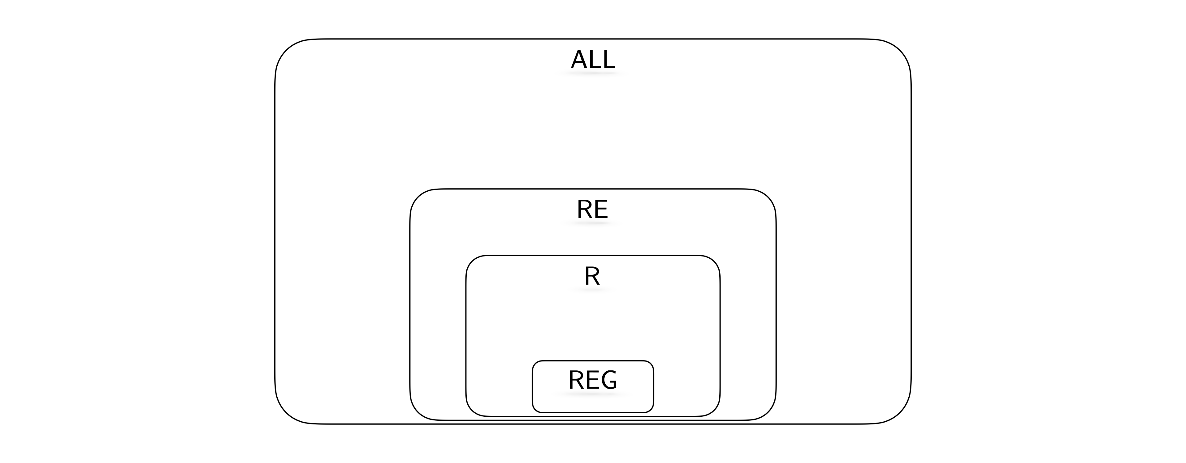
Furthermore, we know \(\{{\texttt{0}}^n {\texttt{1}}^n : n \in \mathbb N\}\) is decidable, but not regular. Therefore we know that the first inclusion above is strict. We will next investigate whether the other inclusions are strict or not.
What are the 7 components in the formal definition of a Turing machine?
True or false: It is possible that in the definition of a TM, \(\Sigma = \Gamma\), where \(\Sigma\) is the input alphabet, and \(\Gamma\) is the tape alphabet.
True or false: On every valid input, any TM either accepts or rejects.
In the 7-tuple definition of a TM, the tape does not appear. Why is this the case?
What is the set of all possible inputs for a TM \(M = (Q, \Sigma, \Gamma, \delta, q_0, q_\text{acc}, q_\text{rej})\)?
In the definition of a TM, the number of states is restricted to be finite. What is the reason for this restriction?
State 4 differences between TMs and DFAs.
True or false: Consider a TM such that the starting state \(q_0\) is also the accepting state \(q_\text{acc}\). It is possible that this TM does not halt on some inputs.
Let \(D = (Q, \Sigma, \delta, q_0, F)\) be a DFA. Define a decider TM \(M\) (specifying the components of the 7-tuple) such that \(L(M) = L(D)\).
What are the 3 components of a configuration of a Turing machine? How is a configuration typically written?
True or false: We say that a language \(K\) is a decidable language if there exists a Turing machine \(M\) such that \(K = L(M)\).
What is a decider TM?
True or false: For each decidable language, there is exactly one TM that decides it.
What do we mean when we say “a high-level description of a TM”?
What is a universal TM?
True or false: A universal TM is a decider.
What is the Church-Turing thesis?
What is the significance of the Church-Turing thesis?
True or false: \(L \subseteq \Sigma^*\) is undecidable if and only if \(\Sigma^* \backslash L\) is undecidable.
Is the following statement true, false, or hard to determine with the knowledge we have so far? \(\varnothing\) is decidable.
Is the following statement true, false, or hard to determine with the knowledge we have so far? \(\Sigma^*\) is decidable.
Is the following statement true, false, or hard to determine with the knowledge we have so far? The language \(\{\left \langle M \right\rangle : \text{$M$ is a TM with $L(M) \neq \varnothing$}\}\) is decidable.
True or false: Let \(L \subseteq \{{\texttt{0}},{\texttt{1}}\}^*\) be defined as follows: \[L = \begin{cases} \{{\texttt{0}}^n{\texttt{1}}^n : n \in \mathbb N\} & \text{if the Goldbach conjecture is true;} \\ \{{\texttt{1}}^{2^n} : n \in \mathbb N\} & \text{otherwise.} \end{cases}\] \(L\) is decidable. (Feel free to Google what Goldbach conjecture is.)
Let \(L\) and \(K\) be two languages. What does “\(L\) reduces to \(K\)” mean? Give an example of \(L\) and \(K\) such that \(L\) reduces to \(K\).
Here are the important things to keep in mind from this chapter.
Understand the key differences and similarities between DFAs and TMs are.
Given a TM, describe in English the language that it solves.
Given the description of a decidable language, come up with a TM that decides it. Note that there are various ways we can describe a TM (what we refer to as the low level, medium level, and the high level representations). You may need to present a TM in any of these levels.
What is the definition of a configuration and why is it important?
The TM computational model describes a very simple programming language.
Even though the definition of a TM is far simpler than any other programming language that you use, convince yourself that it is powerful enough to capture any computation that can be expressed in your favorite programming language. This is a fact that can be proved formally, but we do not do so since it would be extremely long and tedious.
What is the Church-Turing thesis and what does it imply? Note that we do not need to invoke the Church-Turing thesis for the previous point. The Church-Turing thesis is a much stronger claim. It captures our belief that any kind of algorithm that can be carried out by any kind of a natural process can be simulated on a Turing machine. This is not a mathematical statement that can be proved but rather a statement about our universe and the laws of physics.
The set of Turing machines is encodable (i.e. every TM can be represented using a finite-length string). This implies that an algorithm (or Turing machine) can take as input (the encoding of) another Turing machine. This idea is the basis for the universal Turing machine. It allows us to have one (universal) machine/algorithm that can simulate any other machine/algorithm that is given as input.
This chapter contains several algorithms that take encodings of DFAs as input. So these are algorithms that take as input the text representations of other algorithms. There are several interesting questions that one might want to answer given the code of an algorithm (i.e. does it accept a certain input, do two algorithms with different representations solve exactly the same computational problem, etc.) We explore some of these questions in the context of DFAs. It is important you get used to the idea of treating code (which may represent a DFA or a TM) as data/input.
This chapter also introduces the idea of a reduction (the idea of solving a computational problem by using, as a helper function, an algorithm that solves a different problem). Reductions will come up again in future chapters, and it is important that you have a solid understanding of what it means.