The right language and mathematical model to analyze/study randomization is probability theory. The goal of this chapter is to remind you the basic definitions and theorems in the area of discrete probability theory.
A finite probability space is a tuple \((\Omega, \Pr)\), where
\(\Omega\) is a non-empty finite set called the sample space;
\(\Pr : \Omega \to [0,1]\) is a function, called the probability distribution, with the property that \(\sum_{\ell \in \Omega} \Pr[\ell] = 1\).
The elements of \(\Omega\) are called outcomes or samples. If \(\Pr[\ell] = p\), then we say that the probability of outcome \(\ell\) is \(p\).
The probabilities sum to \(1\) by convention. We could have defined it so that they sum to \(100\), and think of probabilities in terms of percentages. Or we could have defined it so they sum to some other value. What is important is that a consistent choice is made. Note that the choice of \(1\) allows us to think of probabilities as fractions, and it is arguably the most natural choice.
The abstract definition above of a finite probability space helps us to mathematically model and reason about situations involving randomness and uncertainties (these situations are often called “random experiments” or just “experiments”). For example, consider the experiment of flipping a single coin. We model this as follows. We let \(\Omega = \{\text{Heads}, \text{Tails}\}\) and we define function \(\Pr\) such that \(\Pr[\text{Heads}] = 1/2\) and \(\Pr[\text{Tails}] = 1/2\). This corresponds to our intuitive understanding that the probability of seeing the outcome Heads is \(1/2\) and the probability of seeing the outcome Tails is also \(1/2\).
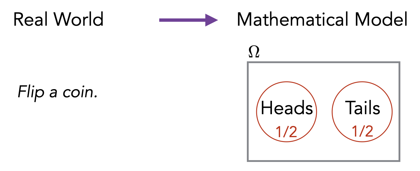
If we flip two coins, the sample space would look as follows (H represents “Heads” and T represents “Tails”).
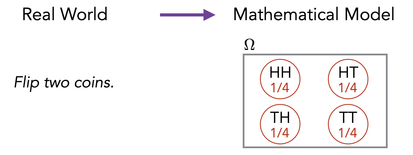
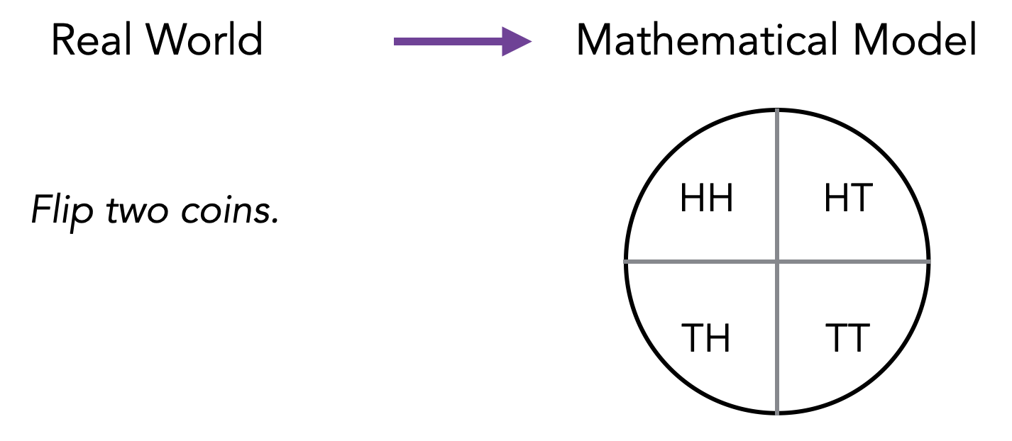
One can visualize the probability space as a circle or pie with area 1. Each outcome gets a slice of the pie proportional to its probability.
In this course, we’ll usually restrict ourselves to finite sample spaces. In cases where we need a countably infinite \(\Omega\), the above definition will generalize naturally.
How would you model a roll of a single \(6\)-sided die using Definition (Finite probability space, sample space, probability distribution)? How about a roll of two dice? How about a roll of a die and a coin toss together?
For the case of a single 6-sided die, we want the model to match our intuitive understanding and real-world experience that the probability of observing each of the possible die rolls \(1, 2, \dots, 6\) is equal. We formalize this by defining the sample space \(\Omega\) and the probability distribution \(\Pr\) as follows: \[\Omega = \{1,2,3,4,5,6\}, \qquad \Pr[\ell] = \dfrac{1}{6} \; \text{ for all } \ell \in \Omega.\]
Similarly, to model a roll of two dice, we can let each outcome be an ordered pair representing the roll of each of the two dice: \[\Omega = \{1,2,3,4,5,6\} \times \{1,2,3,4,5,6\}, \qquad \Pr[\ell] = \left(\dfrac{1}{6}\right)^2 = \dfrac{1}{36} \; \text{ for all } \ell \in \Omega.\]
Lastly, to model a roll of a die and a coin toss together, we can let each outcome be an ordered pair where the first element represents the result of the die roll, and the second element represents the result of the coin toss: \[\Omega = \{1,2,3,4,5,6\} \times \{\text{Heads},\text{Tails}\}, \qquad \Pr[\ell] = \dfrac{1}{6} \cdot \dfrac{1}{2} = \dfrac{1}{12} \; \text{ for all } \ell \in \Omega.\]
Sometimes, the modeling of a real-world random experiment as a probability space can be non-trivial or tricky. It helps a lot to have a step in between where you first go from the real-world experiment to computer code/algorithm (that makes calls to random number generators), and then you define your probability space based on the computer code. In this course, we allow our programs to have access to the functions \(\text{Bernoulli}(p)\) and \(\text{RandInt}(n)\). The function \(\text{Bernoulli}(p)\) takes a number \(0 \leq p \leq 1\) as input and returns \(1\) with probability \(p\) and \(0\) with probability \(1-p\). The function \(\text{RandInt}(n)\) takes a positive integer \(n\) as input and returns a random integer from \(1\) to \(n\) (i.e., every number from \(1\) to \(n\) has probability \(1/n\)). Here is a very simple example of going from a real-world experiment to computer code. The experiment is as follows. You flip a fair coin. If it’s heads, you roll a \(3\)-sided die. If it is tails, you roll a \(4\)-sided die. This experiment can be represented as:
    flip = Bernoulli(1/2)
    if flip == 0:
        die = RandInt(3)
    else:
        die = RandInt(4)
If we were to ask “What is the probability that you roll a 3 or higher?”, this would correspond to asking what is the probability that after the above code is executed, the variable named die stores a value that is 3 or higher.
One advantage of modeling with randomized code is that if there is any ambiguity in the description of the random (real-world) experiment, then it would/should be resolved in this step of creating the randomized code.
The second advantage is that it allows you to easily imagine a probability tree associated with the randomized code. The probability tree gives you clear picture on what the sample space is and how to compute the probabilities of the outcomes. The probability tree corresponding to the above code is as follows.
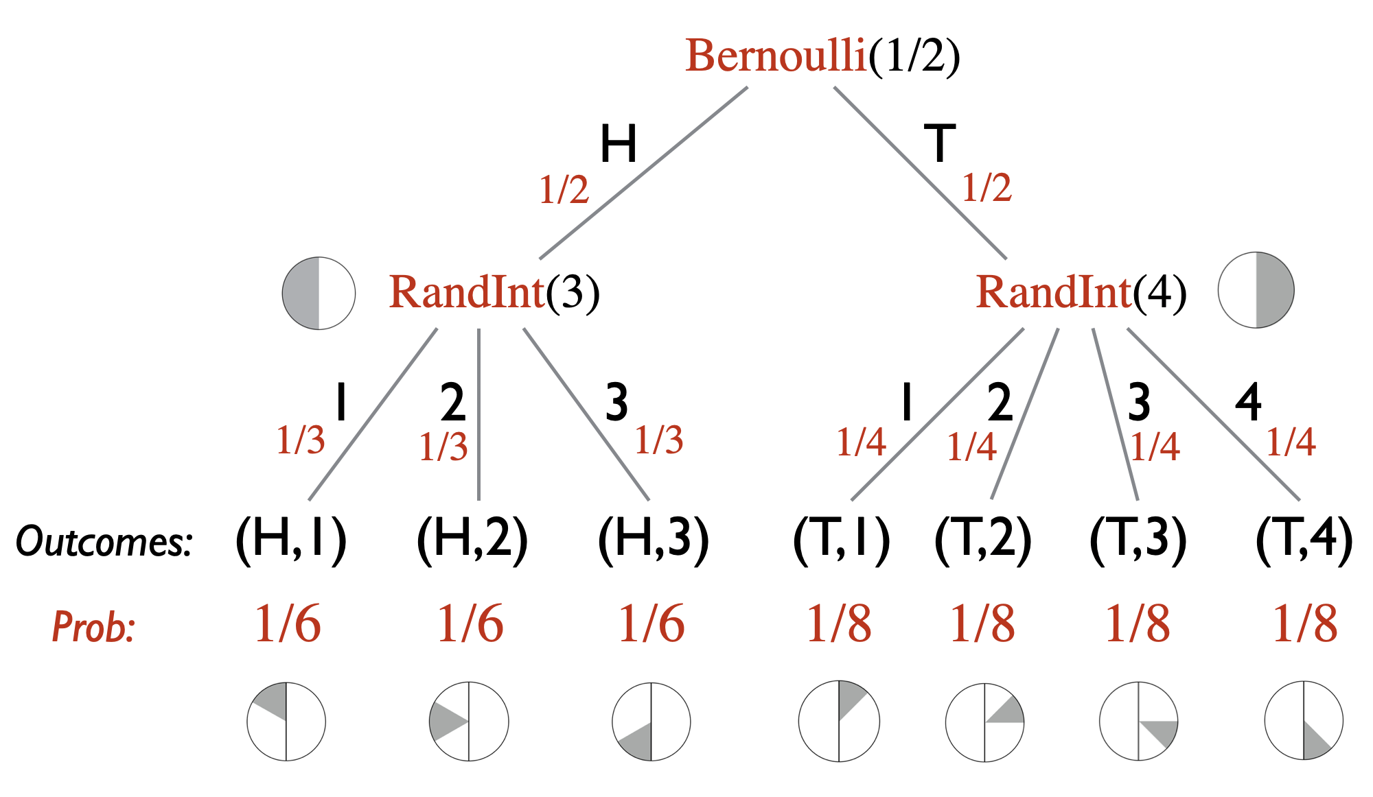
This simple example may not illustrate the usefulness of having a computer code representation of the random experiment, but one can appreciate its value with more sophisticated examples and we do encourage you to think of random experiments as computer code: \[\text{real-world experiment} \longrightarrow \text{computer code / probability tree} \longrightarrow \text{probability space } (\Omega, \Pr).\]
If a probability distribution \(\Pr : \Omega \to [0,1]\) is such that \(\Pr[\ell] = 1/|\Omega|\) for all \(\ell \in \Omega\), then we call it a uniform distribution.
Let \((\Omega, \Pr)\) be a probability space. Any subset of outcomes \(E \subseteq \Omega\) is called an event. We extend the \(\Pr[\cdot]\) notation and write \(\Pr[E]\) to denote \(\sum_{\ell \in E} \Pr[\ell]\). Using this notation, \(\Pr[\varnothing] = 0\) and \(\Pr[\Omega] = 1\). We use the notation \(\overline{E}\) to denote the event \(\Omega \backslash E\).
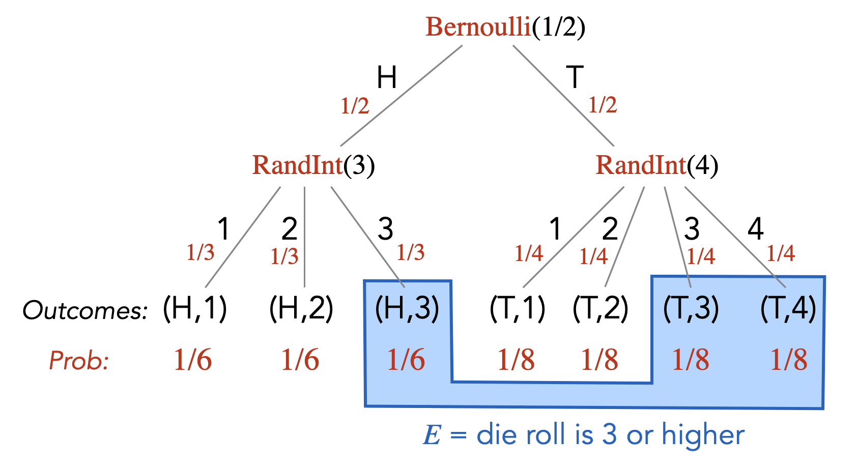
Continuing the example given in Note (Modeling through randomized code), we can define the event \(E = \{(H,3), (T,3), (T,4)\}\). In other words, \(E\) can be described as “die roll is \(3\) or higher”. The probability of \(E\), \(\Pr[E]\), is equal to \(1/6 + 1/8 + 1/8 = 5/12\).
Suppose we roll two \(6\)-sided dice. How many events are there? Write down the event corresponding to “we roll a double” and determine its probability.
Suppose we roll a \(3\)-sided die and see the number \(d\). We then roll a \(d\)-sided die. How many different events are there? Write down the event corresponding to “the second roll is a \(2\)” and determine its probability.
Part (1): We use the model for rolling two 6-sided dice as in Exercise (Probability space modeling). Since an event is any subset of outcomes \(E \subseteq \Omega\), the number of events is the number of such subsets, which is \(|\wp(\Omega)| = 2^{|\Omega|} = 2^{36}\) (here \(\wp(\Omega)\) denotes the power set of \(\Omega\)).
The event corresponding to “we roll a double” can be expressed as \[E = \big\{(\ell,\ell) : \ell \in \{1,2,3,4,5,6\}\big\}\] which has probability \[\Pr[E] = \sum_{\ell \in E}\Pr[\ell] = \dfrac{1}{36} \cdot |E| = \dfrac{6}{36} = \dfrac{1}{6}.\]
Part(2): We model the two dice rolls as follows: \[\Omega = \big\{(a,b) \in \{1,2,3\}^2 : a \geq b\big\}, \qquad \Pr[(a,b)] = \dfrac{1}{3} \cdot \dfrac{1}{a} = \dfrac{1}{3a}.\] The restriction that \(a \geq b\) is imposed because the second die depends on the first roll and the result of the second roll cannot be larger than that of the first. Note that we could also have used a model where \(\Omega = \{1,2,3\}^2\) and assigned a probability of 0 to the outcomes where \(a < b\), but considering outcomes that never occur is typically not very useful.
In the model we originally defined, the number of events is \(|\wp(\Omega)| = 2^{|\Omega|} = 2^6 = 64\). Note that the number of events depends on the size of the sample space, so this number can vary depending on the model.
The event corresponding to “the second roll is a 2” is given by \[E = \{(a,b) \in \Omega : b = 2\} = \{(2,2),(3,2)\}\] which has probability \[\Pr[E] = \sum_{\ell \in E}\Pr[\ell] = \Pr[(2,2)] + \Pr[(3,2)] = \dfrac{1}{3\cdot2} + \dfrac{1}{3\cdot3} = \dfrac{5}{18}.\]
Let \(A\) and \(B\) be two events. Prove the following.
If \(A \subseteq B\), then \(\Pr[A] \leq \Pr[B]\).
\(\Pr[\overline{A}] = 1 - \Pr[A]\).
\(\Pr[A \cup B] = \Pr[A] + \Pr[B] - \Pr[A \cap B]\).
Part (1): Suppose \(A \subseteq B\). Recall that \(\Pr\) is a non-negative function (i.e. \(\Pr[\ell] \geq 0\) for all \(\ell \in \Omega\)). Hence,
\[\begin{aligned} \Pr[A] &= \sum_{\ell \in A}\Pr[\ell] &\text{by the definition of event} \\ &\leq \sum_{\ell \in A}\Pr[\ell] + \sum_{\ell \in B \setminus A}\Pr[\ell] &\text{by non-negativity of $\Pr$} \\ &= \sum_{\ell \in B}\Pr[\ell] & \\ &= \Pr[B]. & \\\end{aligned}\]
Part (2): Recall that \(\overline{A}\) denotes \(\Omega \setminus A\), and that \(\sum_{\ell \in \Omega}\Pr[\ell] = 1\). Hence, \[\begin{aligned} \Pr[\overline{A}] &= \sum_{\ell \in \overline{A}}\Pr[\ell] &\text{by definition of event}\\ &= \sum_{\ell \in \Omega \setminus A}\Pr[\ell] \\ &= \sum_{\ell \in \Omega}\Pr[\ell] - \sum_{\ell \in A}\Pr[\ell] \\ &= 1 - \Pr[A] & \text{by definition of prob. distr.}\end{aligned}\]
Part (3) By partitioning \(A \cup B\) into \(A \setminus B\), \(B \setminus A\), and \(A \cap B\), we see that \[\begin{aligned} \Pr[A \cup B] &= \sum_{\ell \in A \cup B}\Pr[\ell] \quad \text{by definition of event} \\ &= \sum_{\ell \in A \setminus B}\Pr[\ell] + \sum_{\ell \in B \setminus A}\Pr[\ell] + \sum_{\ell \in A \cap B}\Pr[\ell] \\ &= \left(\sum_{\ell \in A}\Pr[\ell] - \sum_{\ell \in A \cap B}\Pr[\ell]\right) + \left(\sum_{\ell \in B}\Pr[\ell] - \sum_{\ell \in A \cap B}\Pr[\ell]\right) + \sum_{\ell \in A \cap B}\Pr[\ell] \\ &= \sum_{\ell \in A}\Pr[\ell] + \sum_{\ell \in B}\Pr[\ell]- \sum_{\ell \in A \cap B}\Pr[\ell] \\ &= \Pr[A] + \Pr[B] - \Pr[A \cap B] \quad \text{by definition of event.}\end{aligned}\]
We say that two events \(A\) and \(B\) are disjoint events if \(A \cap B = \varnothing\).
Let \(A_1,A_2,\ldots,A_n\) be events. Then \[\Pr[A_1 \cup A_2 \cup \cdots \cup A_n] \leq \Pr[A_1] + \Pr[A_2] + \cdots + \Pr[A_n].\] We get equality if and only if the \(A_i\)’s are pairwise disjoint.
By the last part of Exercise (Basic facts about probability), we can conclude that \[\Pr[A \cup B] \leq \Pr[A] + \Pr[B].\] We also notice that equality holds if and only if \(\Pr[A \cap B] = 0\), which happens if and only if \(A\) and \(B\) are disjoint. We will extend this by induction on \(n\).
The expression is identical on both sides for the case where \(n = 1\), and the case where \(n = 2\) is exactly as above. These serve as the base cases for our induction.
For the inductive case, assume the proposition holds true for \(n = k\). We seek to show that it too holds true for \(n = k+1\). Given events \(A_1, A_2, \dots, A_k, A_{k+1}\), let \[A = A_1 \cup A_2 \cup \cdots \cup A_k, \qquad B = A_{k+1}.\] Then \[\begin{aligned} \Pr[A_1 \cup A_2 \cup \cdots \cup A_k \cup A_{k+1}] &= \Pr[A \cup B] \\ &\leq \Pr[A] + \Pr[B] \quad \text{by the above result} \\ &= \Pr[A_1 \cup A_2 \cup \cdots \cup A_k] + \Pr[A_{k+1}] \\ &\leq \left(\Pr[A_1] + \cdots + \Pr[A_k]\right) + \Pr[A_{k+1}] \quad \text{by IH}\end{aligned}\] where equality holds if and only if \(A\) and \(B\) are disjoint and \(A_1, \dots, A_k\) are pairwise disjoint. In other words, equality holds if and only if \[\bigcup_{t=1}^{k} (A_{t} \cap A_{k+1}) = \varnothing \qquad \text{ and } \qquad A_i \cap A_j = \varnothing\text{ for all }1 \leq i < j \leq k,\] which in turn holds if and only if \[A_i \cap A_j = \varnothing\text{ for all }1 \leq i < j \leq k+1.\] (i.e. \(A_1, \dots, A_{k+1}\) are pairwise disjoint). This completes the proof.
Let \(E\) be an event with \(\Pr[E] \neq 0\). The conditional probability of outcome \(\ell \in \Omega\) given \(E\), denoted \(\Pr[\ell \; | \;E]\), is defined as \[\Pr[\ell \; | \;E] = \begin{cases} 0 &\text{if $\ell \not \in E$}\\ \frac{\Pr[\ell]}{\Pr[E]} &\text{if $\ell \in E$} \end{cases}\] For an event \(A\), the conditional probability of \(A\) given \(E\), denoted \(\Pr[A \; | \;E]\), is defined as \[\begin{aligned} \Pr[A \; | \;E] = \frac{\Pr[A \cap E]}{\Pr[E]}.\end{aligned}\]
Once again, continuing the example given in Note (Modeling through randomized code), let \(E\) be the event that the die roll is \(3\) or higher. Then for each outcome of the sample space, we can calculate its probability, given the event \(E\).
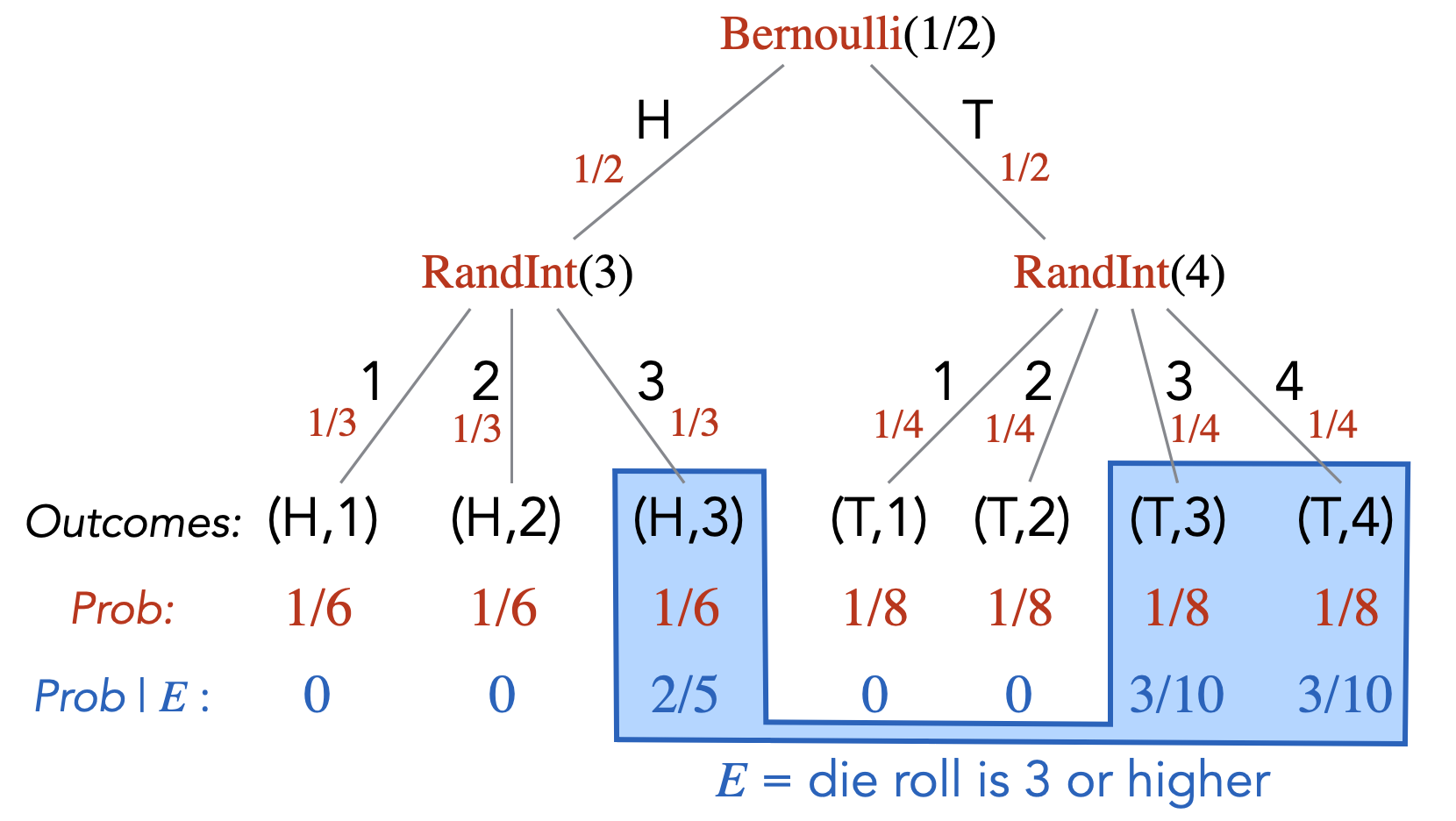
For example, \(\Pr[(H,1) \; | \;E] = 0\) and \(\Pr[(H,3) \; | \;E] = 2/5\). We can also calculate the conditional probabilities of events. Let \(A\) be the event that the coin toss resulted in Tails. Then \(\Pr[A \; | \;E] = 3/10 + 3/10 = 3/5\).
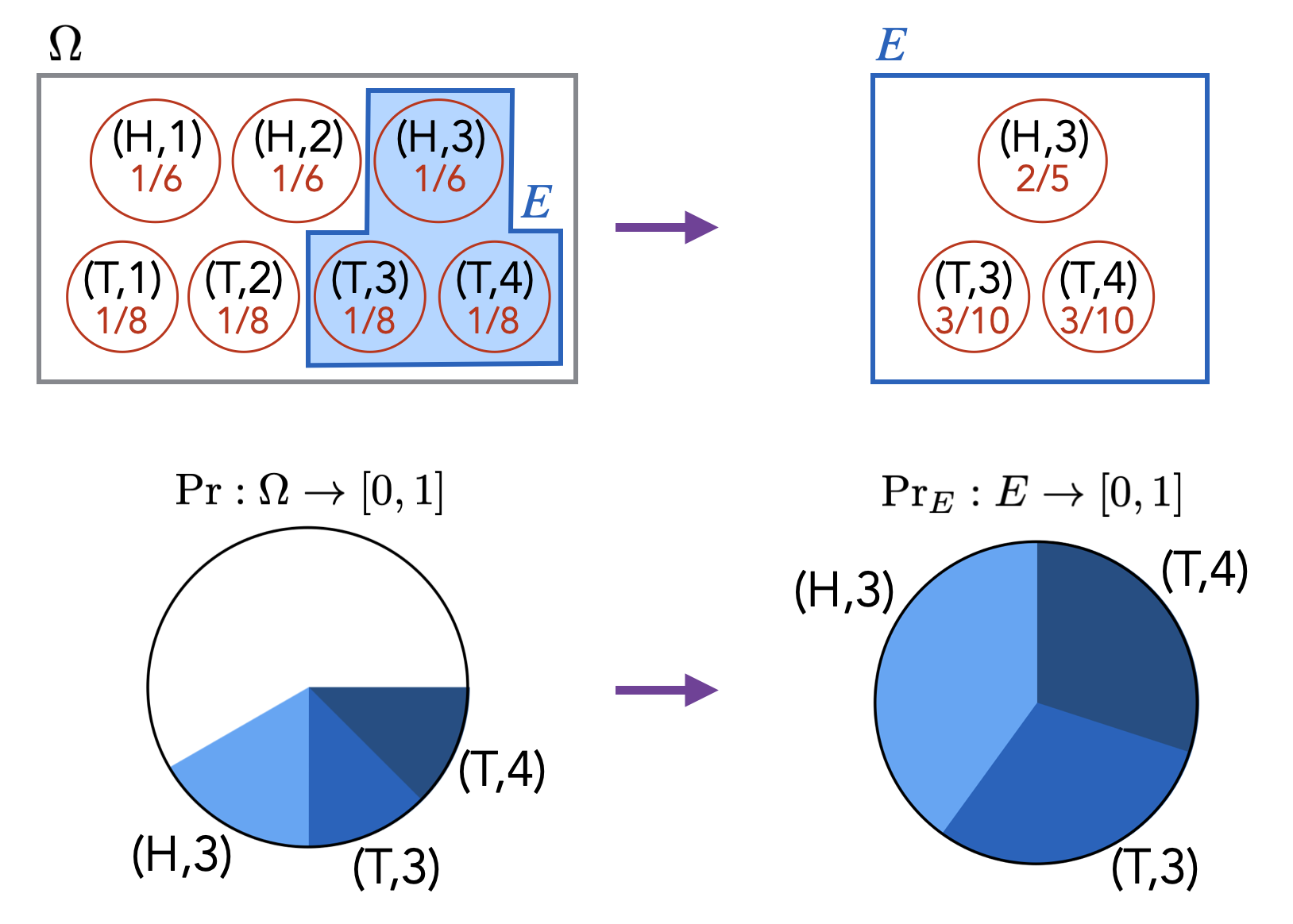
Although it may not be immediately obvious, the above definition of conditional probability does correspond to our intuitive understanding of what conditional probability should represent. If we are told that event \(E\) has already happened, then we know that the probability of any outcome outside of \(E\) should be \(0\). Therefore, we can view the conditioning on event \(E\) as a transformation of our probability space where we revise the probabilities (i.e., we revise the probability function \(\Pr[\cdot]\)). In particular, the original probability space \((\Omega, \Pr)\) gets transformed to \((\Omega, \Pr_E)\), where \(\Pr_E\) is such that for any \(\ell \not \in E\), we have \(\Pr_E[\ell] = 0\), and for any \(\ell \in E\), we have \(\Pr_E[\ell] = \Pr[\ell] / \Pr[E]\). The \(1/\Pr[E]\) factor here is a necessary normalization factor that ensures the probabilities of all the outcomes sum to \(1\) (which is required by Definition (Finite probability space, sample space, probability distribution)). Indeed, \[\begin{aligned} \textstyle \sum_{\ell \in \Omega} \Pr_E[\ell] & = \textstyle \sum_{\ell \not \in E} \Pr_E[\ell] + \sum_{\ell \in E} \Pr_E[\ell] \\ & = \textstyle 0 + \sum_{\ell \in E} \Pr[\ell]/\Pr[E] \\ & = \textstyle \frac{1}{\Pr[E]} \sum_{\ell \in E} \Pr[\ell] \\ & = 1.\end{aligned}\] If we are interested in the event “\(A\) given \(E\)” (denoted by \(A \; | \;E\)) in the probability space \((\Omega, \Pr)\), then we are interested in the event \(A\) in the probability space \((\Omega, \Pr_E)\). That is, \(\Pr[A \; | \;E] = \Pr_E[A]\). Therefore, \[\textstyle \Pr[A \; | \;E] = \Pr_E[A] = \Pr_E[A \cap E] = \displaystyle \frac{\Pr[A \cap E]}{\Pr[E]},\] where the last equality holds by the definition of \(\Pr_E[ \cdot ]\). We have thus recovered the equality in Definition (Conditional probability).
Conditioning on event \(E\) can also be viewed as redefining the sample space \(\Omega\) to be \(E\), and then renormalizing the probabilities so that \(\Pr[\Omega] = \Pr[E] = 1\).
Suppose we roll a \(3\)-sided die and see the number \(d\). We then roll a \(d\)-sided die. We are interested in the probability that the first roll was a \(1\) given that the second roll was a \(1\). First express this probability using the notation of conditional probability and then determine what the probability is.
We use the model defined in Exercise (Practice with events). The event that the first roll is a 1 is \[E_1 = \{(1,1)\}\] and the event that the second roll is a 1 is \[E_2 = \{(1,1),(2,1),(3,1)\}\] with corresponding probabilities \[\Pr[E_1] = \dfrac{1}{3}, \qquad \Pr[E_2] = \dfrac{1}{3\cdot1} + \dfrac{1}{3\cdot2} + \dfrac{1}{3\cdot3} = \dfrac{11}{18}.\] Then the conditional probability we are interested in is \[\Pr[E_1 \mid E_2] = \dfrac{\Pr[E_1 \cap E_2]}{\Pr[E_2]} = \dfrac{\Pr[E_1]}{\Pr[E_2]} = \dfrac{1/3}{11/18} = \dfrac{6}{11}.\]
Let \(n \geq 2\) and let \(A_1,A_2,\ldots,A_n\) be events. Then \[\begin{aligned} & \Pr[A_1 \cap \cdots \cap A_n] = \\ & \qquad \Pr[A_1] \cdot \Pr[A_2 \; | \;A_1] \cdot \Pr[A_3 \; | \;A_1 \cap A_2] \cdots \Pr[A_n \; | \;A_1 \cap A_2 \cap \cdots \cap A_{n-1}].\end{aligned}\]
We prove the proposition by induction on \(n\). The base case with two events follows directly from the definition of conditional probability. Let \(A = A_n\) and \(B = A_1 \cap \ldots \cap A_{n-1}\). Then \[\begin{aligned} \Pr[A_1\cap \cdots \cap A_n] & = \Pr[A \cap B] \\ &= \Pr[B] \cdot \Pr[A \; | \;B] \\ &= \Pr[A_1 \cap \cdots \cap A_{n-1}] \cdot \Pr[A_n \; | \;A_1 \cap \cdots \cap A_{n-1}],\end{aligned}\] where we used the definition of conditional probability for the second equality. Applying the induction hypothesis to \(\Pr[A_1 \cap \cdots \cap A_{n-1}]\) gives the desired result.
Suppose there are 100 students in 15-251 and 5 of the students are Andrew Yang supporters. We pick 3 students from class uniformly at random. Calculate the probability that none of them are Andrew Yang supporters using Proposition (Chain rule).
For \(i = 1,2,3\), let \(A_i\) be the event that the \(i\)’th student we pick is not a Andrew Yang supporter. Then using the chain rule, the probability that none of them are Andrew Yang supporters is \[\Pr[A_1 \cap A_2 \cap A_3] = \Pr[A_1] \cdot \Pr[A_2 \mid A_1] \cdot \Pr[A_3 \mid A_1 \cap A_2] = \dfrac{95}{100} \cdot \dfrac{94}{99} \cdot \dfrac{93}{98}.\]
Let \(A\) and \(B\) be two events. We say that \(A\) and \(B\) are independent events if \(\Pr[A \cap B] = \Pr[A]\cdot \Pr[B]\). Note that if \(\Pr[B] \neq 0\), then this is equivalent to \(\Pr[A \; | \;B] = \Pr[A]\). If \(\Pr[A] \neq 0\), it is also equivalent to \(\Pr[B \; | \;A] = \Pr[B]\).
Let \(A_1, A_2,\ldots, A_n\) be events. We say that \(A_1,\ldots,A_n\) are independent if for any subset \(S \subseteq \{1,2,\ldots,n\}\), \[\Pr\left[\bigcap_{i \in S} A_i\right] = \prod_{i\in S} \Pr[A_i].\]
Above we have given the definition of independent events as presented in 100% of the textbooks on probability theory. Yet, there is something deeply unsatisfying about this definition. In many situations people want to compute a probability of the form \(\Pr[A \cap B]\), and if possible (if they are independent), would like to use the equality \(\Pr[A \cap B] = \Pr[A] \Pr[B]\) to simplify the calculation. In order to do this, they will informally argue that events \(A\) and \(B\) are independent in the intuitive sense of the word. For example, they argue that if \(B\) happens, then this doesn’t affect the probability of \(A\) happening (this argument is not done by calculation, but by informal argument). Then using this, they justify using the equality \(\Pr[A \cap B] = \Pr[A] \Pr[B]\) in their calculations. So really, secretly, people are not using Definition (Independent events) but some other non-formal intuitive definition of independence, and then concluding what the formal definition says, which is \(\Pr[A \cap B] = \Pr[A] \Pr[B]\).
To be a bit more explicit, recall that the approach to answering probability related questions is to go from a real-world experiment we want to analyze to a formal probability space model: \[\text{real-world experiment} \longrightarrow \text{probability space } (\Omega, \Pr).\] People often argue the independence of events \(A\) and \(B\) on the left-hand-side in order to use \(\Pr[A \cap B] = \Pr[A] \Pr[B]\) on the right-hand-side. The left-hand-side, however, is not really a formal setting and may have ambiguities. And why does our intuitive notion of independence allow us to conclude \(\Pr[A \cap B] = \Pr[A] \Pr[B]\)? In these situations, it helps to add the “computer code” step in between: \[\text{real-world experiment} \longrightarrow \text{computer code} \longrightarrow \text{probability space } (\Omega, \Pr).\] Computer code has no ambiguities and we can give a formal definition of independence using it. Suppose you have a randomized code modeling the real-world experiment, and suppose that you can divide the code into two separate parts. Suppose \(A\) is an event that depends only on the first part of the code, and \(B\) is an event that depends only on the second part of the code. If you can prove that the two parts of the code cannot affect each other, then we say that \(A\) and \(B\) are independent. When \(A\) and \(B\) are independent in this sense, then one can verify that indeed the equality \(\Pr[A \cap B] = \Pr[A] \Pr[B]\) holds.
A random variable is a function \(\mathbf{X} : \Omega \to \mathbb R\), where \(\Omega\) is a sample space.
Note that a random variable is just a labeling of the elements in \(\Omega\) with some real numbers. One can think of this as a transformation of the original sample space into one that contains only numbers. For example, suppose the original sample space corresponds to flipping two coins. Then we can define a random variable \(\mathbf{X}\) which maps an outcome in the sample space to the number of tails in the outcome. Since we are only flipping two coins, the possible outputs of \(\mathbf{X}\) are \(0\), \(1\), and \(2\).
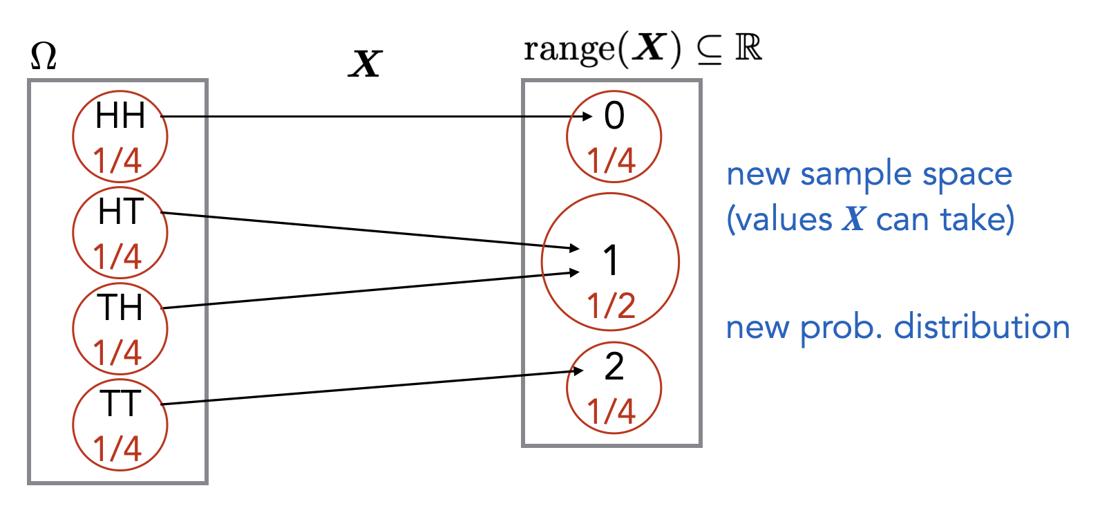
This kind of transformation is often desirable. For example, the transformation allows us to take a weighted average of the elements in the new sample space, where the weights correspond to the probabilities of the elements (if the distribution is uniform, the weighted average is just the regular average). This is called the expectation of the random variable and is formally defined below in Definition (Expected value of a random variable). Without this transformation into real numbers, the concept of an “expected value” (i.e. averaging) would not be possible to define.
Almost always, the random variables we consider in this course will have a range that is a subset of \(\mathbb N\).
Let \(\mathbf{X}\) be a random variable and \(x \in \mathbb R\) be some real value. We use \[\begin{aligned} \mathbf{X}=x & \quad \text{ to denote the event $\{\ell \in \Omega : \mathbf{X}(\ell) = x \}$},\\ \mathbf{X} \leq x & \quad \text{ to denote the event $\{\ell \in \Omega : \mathbf{X}(\ell) \leq x \}$},\\ \mathbf{X} \geq x & \quad \text{ to denote the event $\{\ell \in \Omega : \mathbf{X}(\ell) \geq x \}$},\\ \mathbf{X} < x & \quad \text{ to denote the event $\{\ell \in \Omega : \mathbf{X}(\ell) < x \}$},\\ \mathbf{X} > x & \quad \text{ to denote the event $\{\ell \in \Omega : \mathbf{X}(\ell) > x \}$}.\end{aligned}\] For example, \(\Pr[\mathbf{X}=x]\) denotes \(\Pr[\{\ell \in \Omega : \mathbf{X}(\ell) = x\}]\). More generally, for \(S \subseteq \mathbb R\), we use \[\begin{aligned} \mathbf{X} \in S & \quad \text{ to denote the event $\{\ell \in \Omega : \mathbf{X}(\ell) \in S \}$}.\end{aligned}\]
Suppose we roll two \(6\)-sided dice. Let \(\mathbf{X}\) be the random variable that denotes the sum of the numbers we see. Explicitly write down the input-output pairs for the function \(\mathbf{X}\). Calculate \(\Pr[\mathbf{X} \geq 7]\).
We use the model for rolling two 6-sided dice as in Exercise (Probability space modeling). Then \[\begin{array}{llllll} {\mathbf{X}}(1,1) = 2, & {\mathbf{X}}(1,2) = 3, & {\mathbf{X}}(1,3) = 4, & {\mathbf{X}}(1,4) = 5, & {\mathbf{X}}(1,5) = 6, & {\mathbf{X}}(1,6) = 7, \\ {\mathbf{X}}(2,1) = 3, & {\mathbf{X}}(2,2) = 4, & {\mathbf{X}}(2,3) = 5, & {\mathbf{X}}(2,4) = 6, & {\mathbf{X}}(2,5) = 7, & {\mathbf{X}}(2,6) = 8, \\ {\mathbf{X}}(3,1) = 4, & {\mathbf{X}}(3,2) = 5, & {\mathbf{X}}(3,3) = 6, & {\mathbf{X}}(3,4) = 7, & {\mathbf{X}}(3,5) = 8, & {\mathbf{X}}(3,6) = 9, \\ {\mathbf{X}}(4,1) = 5, & {\mathbf{X}}(4,2) = 6, & {\mathbf{X}}(4,3) = 7, & {\mathbf{X}}(4,4) = 8, & {\mathbf{X}}(4,5) = 9, & {\mathbf{X}}(4,6) = 10, \\ {\mathbf{X}}(5,1) = 6, & {\mathbf{X}}(5,2) = 7, & {\mathbf{X}}(5,3) = 8, & {\mathbf{X}}(5,4) = 9, & {\mathbf{X}}(5,5) = 10, & {\mathbf{X}}(5,6) = 11, \\ {\mathbf{X}}(6,1) = 7, & {\mathbf{X}}(6,2) = 8, & {\mathbf{X}}(6,3) = 9, & {\mathbf{X}}(6,4) = 10, &{\mathbf{X}}(6,5) = 11, & {\mathbf{X}}(6,6) = 12. \end{array}\] Since the probability distribution is uniform over the outcomes, \[\Pr[{\mathbf{X}} \geq 7] = \dfrac{1}{36} \cdot |\{\ell \in \Omega : {\mathbf{X}}(\ell) \geq 7\}| = \dfrac{1}{36} \cdot 21 = \dfrac{7}{12}.\]
Using the randomized code and probability tree point of view, we can simply define a random variable as a numerical variable in some randomized code (more accurately, the variable’s value at the end of the execution of the code). For example, consider the following randomized code.
    S = RandInt(6) + RandInt(6)
    if S == 12:
        I = 1
    else:
        I = 0
Here we have two random variables corresponding to the variables in the code, \(\mathbf{S}\) and \(\mathbf{I}\). From the probability tree picture, we can see how these two random variables can be viewed as functions from the sample space (the set of leaves) to \(\mathbb R\) since they map each leaf/outcome to some numerical value.
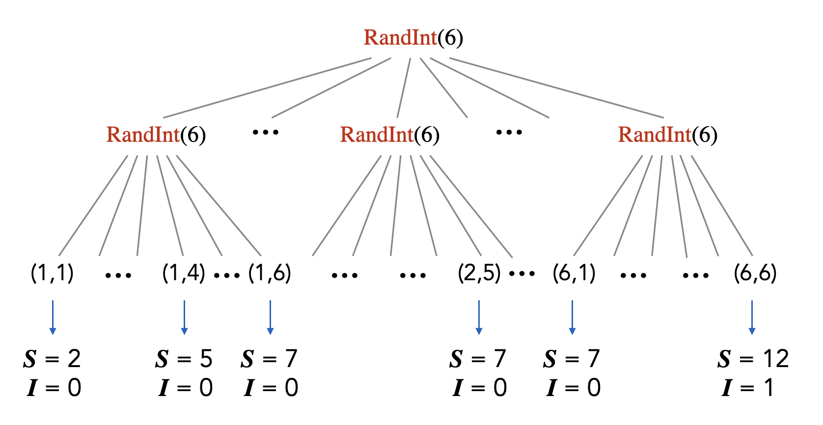
Given some probability space \((\Omega, \Pr)\) and a random variable \(\mathbf{X} : \Omega \to \mathbb R\), we often forget about the original sample space and consider the sample space to be the range of \(\mathbf{X}\), \(\text{range}(\mathbf{X}) = \{\mathbf{X}(\ell): \ell \in \Omega\}\).
Let \(\mathbf{X} : \Omega \to \mathbb R\) be a random variable. The probability mass function (PMF) of \(\mathbf{X}\) is a function \(p_{\mathbf{X}} : \mathbb R\to [0,1]\) such that for any \(x \in \mathbb R\), \(p_{\mathbf{X}}(x) = \Pr[\mathbf{X} = x]\).
Related to the previous remark, we sometimes “define” a random variable by just specifying its probability mass function. In particular, we make no mention of the underlying sample space.
Let \(\mathbf{X}\) be a random variable. The expected value of \(\mathbf{X}\), denoted \(\mathbb E[\mathbf{X}]\), is defined as follows: \[\mathbb E[\mathbf{X}] = \sum_{\ell \in \Omega} \Pr[\ell]\cdot \mathbf{X}(\ell).\] Equivalently, \[\mathbb E[\mathbf{X}] = \sum_{x \in \text{range}(\mathbf{X})} \Pr[\mathbf{X}=x]\cdot x,\] where \(\text{range}(\mathbf{X}) = \{\mathbf{X}(\ell): \ell \in \Omega\}\).
Prove that the above two expressions for \(\mathbb E[\mathbf{X}]\) are equivalent.
We show a chain of equalities from the RHS to the LHS: \[\begin{aligned} \sum_{x \in \operatorname{range}({\mathbf{X}})}\Pr[{\mathbf{X}} = x] \cdot x &= \sum_{x \in \operatorname{range}({\mathbf{X}})}\Pr[\{\ell \in \Omega : {\mathbf{X}}(\ell) = x\}] \cdot x \\ &= \sum_{x \in \operatorname{range}({\mathbf{X}})}\sum_{\substack{\ell \in \Omega \\ {\mathbf{X}}(\ell) = x}}\Pr[\ell] \cdot x \\ &= \sum_{x \in \operatorname{range}({\mathbf{X}})}\sum_{\substack{\ell \in \Omega \\ {\mathbf{X}}(\ell) = x}}\Pr[\ell] \cdot {\mathbf{X}}(\ell) \\ &= \sum_{\ell \in \Omega}\Pr[\ell] \cdot {\mathbf{X}}(\ell). \\\end{aligned}\]
Suppose we roll two \(6\)-sided dice. Let \(\mathbf{X}\) be the random variable that denotes the sum of the numbers we see. Calculate \(\mathbb E[\mathbf{X}]\).
We refer to the input-output pairs of \({\mathbf{X}}\) (recall that random variables are functions) in Exercise (Practice with random variables). With a lot of tedious calculations, we can compute \[\mathbb E[{\mathbf{X}}] = \sum_{x \in \operatorname{range}({\mathbf{X}})}\Pr[{\mathbf{X}} = x] \cdot x = \dfrac{1}{36} \cdot 2 + \dfrac{2}{36} \cdot 3 + \dfrac{3}{36} \cdot 4 + \cdots + \dfrac{1}{36} \cdot 12 = 7.\] We will see a less tedious way of performing such calculations in the following exercise.
Let \(\mathbf{X}\) and \(\mathbf{Y}\) be two random variables, and let \(c_1,c_2 \in \mathbb R\) be some constants. Then \[\mathbb E[c_1\mathbf{X}+c_2\mathbf{Y}] = c_1\mathbb E[\mathbf{X}] + c_2\mathbb E[\mathbf{Y}].\]
Define the random variable \(\mathbf{Z}\) as \(\mathbf{Z} = c_1\mathbf{X} + c_2\mathbf{Y}\). Then using the definition of expected value, we have \[\begin{aligned} \mathbb E[c_1\mathbf{X}+c_2\mathbf{Y}] & = \mathbb E[\mathbf{Z}] \\ & = \sum_{\ell \in \Omega} \Pr[\ell]\cdot \mathbf{Z}(\ell) \\ & = \sum_{\ell \in \Omega} \Pr[\ell]\cdot (c_1\mathbf{X}(\ell) + c_2\mathbf{Y}(\ell)) \\ & = \sum_{\ell \in \Omega} \Pr[\ell]\cdot c_1 \mathbf{X}(\ell) + \Pr[\ell] \cdot c_2 \mathbf{Y}(\ell) \\ & = \left(\sum_{\ell \in \Omega} \Pr[\ell]\cdot c_1 \mathbf{X}(\ell)\right ) + \left( \sum_{\ell \in \Omega} \Pr[\ell]\cdot c_2 \mathbf{Y}(\ell)\right) \\ & = c_1 \left(\sum_{\ell \in \Omega} \Pr[\ell]\cdot \mathbf{X}(\ell)\right ) + c_2 \left( \sum_{\ell \in \Omega} \Pr[\ell]\cdot \mathbf{Y}(\ell)\right) \\ & = c_1\mathbb E[\mathbf{X}] + c_2\mathbb E[\mathbf{Y}], \end{aligned}\] as desired.
Let \(\mathbf{X}_1,\mathbf{X}_2,\ldots,\mathbf{X}_n\) be random variables, and \(c_1,c_2,\ldots,c_n \in \mathbb R\) be some constants. Then \[\mathbb E[c_1\mathbf{X}_1 + c_2\mathbf{X}_2 + \cdots + c_n\mathbf{X}_n] = c_1\mathbb E[\mathbf{X}_1] + c_2\mathbb E[\mathbf{X}_2] + \cdots + c_n\mathbb E[\mathbf{X}_n].\] In particular, when all the \(c_i\)’s are 1, we get \[\mathbb E[\mathbf{X}_1 + \mathbf{X}_2 + \cdots + \mathbf{X}_n] = \mathbb E[\mathbf{X}_1] + \mathbb E[\mathbf{X}_2] + \cdots + \mathbb E[\mathbf{X}_n].\]
Suppose we roll three \(10\)-sided dice. Let \(\mathbf{X}\) be the sum of the three values we see. Calculate \(\mathbb E[\mathbf{X}]\).
Let \({\mathbf{X}}_1, {\mathbf{X}}_2, {\mathbf{X}}_3\) be the values of the rolls of each of the three dice. Note that \({\mathbf{X}}_1, {\mathbf{X}}_2, {\mathbf{X}}_3\) are random variables and that \({\mathbf{X}} = {\mathbf{X}}_1 + {\mathbf{X}}_2 + {\mathbf{X}}_3\). Then since \({\mathbf{X}}_1, {\mathbf{X}}_2, {\mathbf{X}}_3\) are identically distributed, we can compute \[\begin{aligned} \mathbb E[{\mathbf{X}}_1] = \mathbb E[{\mathbf{X}}_2] = \mathbb E[{\mathbf{X}}_3] &= \sum_{x \in \operatorname{range}({\mathbf{X}}_1)}\Pr[{\mathbf{X}}_1 = x] \cdot x \\ &= \sum_{x=1}^{10}\Pr[{\mathbf{X}}_1 = x] \cdot x &\text{since $\operatorname{range}({\mathbf{X}}_1) = \{1,2,\dots,10\}$}\\ &= \sum_{x=1}^{10}\dfrac{1}{10} \cdot x \\ &= \dfrac{11}{2}\end{aligned}\] and by linearity of expectation, \[\mathbb E[{\mathbf{X}}] = \mathbb E[{\mathbf{X}}_1 + {\mathbf{X}}_2 + {\mathbf{X}}_3] = \mathbb E[{\mathbf{X}}_1] + \mathbb E[{\mathbf{X}}_2] + \mathbb E[{\mathbf{X}}_3] = 3 \cdot \dfrac{11}{2} = \dfrac{33}{2}.\]
Two random variables \(\mathbf{X}\) and \(\mathbf{Y}\) are independent random variables if for all \(x, y \in \mathbb R\), the events \(\mathbf{X}=x\) and \(\mathbf{Y}=y\) are independent. The definition generalizes to more than two random variables analogous to Definition (Independent events).
If \(\mathbf{X}_1,\mathbf{X}_2,\ldots, \mathbf{X}_n\) are independent random variables, then \[\mathbb E[\mathbf{X}_1\mathbf{X}_2\cdots \mathbf{X}_n] = \mathbb E[\mathbf{X}_1] \cdot \mathbb E[\mathbf{X}_2] \cdots \mathbb E[\mathbf{X}_n].\]
We will first show the following sub-claim: if \({\mathbf{X}}\) and \({\mathbf{Y}}\) are independent random variables, then \[\mathbb E[{\mathbf{XY}}] = \mathbb E[{\mathbf{X}}] \cdot \mathbb E[{\mathbf{Y}}].\] Indeed, noting that the events \(({\mathbf{X}} = x) \cap ({\mathbf{Y}} = y)\), for \(x \in \operatorname{range}({\mathbf{X}})\) and \(y \in \operatorname{range}({\mathbf{Y}})\), partition \(\Omega\), \[\begin{aligned} \mathbb E[{\mathbf{XY}}] &= \sum_{x \in \operatorname{range}({\mathbf{X}})}\sum_{y \in \operatorname{range}({\mathbf{Y}})}\mathbb E[{\mathbf{XY}} \; | \;({\mathbf{X}} = x) \cap ({\mathbf{Y}} = y)] \cdot \Pr[({\mathbf{X}} = x) \cap ({\mathbf{Y}} = y)] \\ &= \sum_{x \in \operatorname{range}({\mathbf{X}})}\sum_{y \in \operatorname{range}({\mathbf{Y}})} xy \cdot\Pr[({\mathbf{X}} = x) \cap ({\mathbf{Y}} = y)] \\ &= \sum_{x \in \operatorname{range}({\mathbf{X}})}\sum_{y \in \operatorname{range}({\mathbf{Y}})} xy \cdot\Pr[{\mathbf{X}} = x] \cdot \Pr[{\mathbf{Y}} = y] \\ &= \left(\sum_{x \in \operatorname{range}({\mathbf{X}})} x \cdot \Pr[{\mathbf{X}} = x]\right) \cdot \left(\sum_{y \in \operatorname{range}({\mathbf{Y}})} y \cdot \Pr[{\mathbf{Y}} = y] \right) \\ &= \mathbb E[{\mathbf{X}}] \cdot \mathbb E[{\mathbf{Y}}]. \end{aligned}\] Now, we prove the original statement by induction on \(n\). Both sides are identical for the case where \(n = 1\), and the above claim is exactly the case where \(n = 2\). These are our base cases.
For the inductive case, assume the proposition holds true for \(n = k\). We seek to show that it also holds for \(n = k+1\). Suppose \({\mathbf{X}}_1, {\mathbf{X}}_2, \dots, {\mathbf{X}}_{k+1}\) are independent random variables. Let \({\mathbf{X}} = \prod_{j=1}^{k}{\mathbf{X}}_j\) and \({\mathbf{Y}} = {\mathbf{X}}_{k+1}\). We have \[\begin{aligned} \mathbb E\left[\prod_{j=1}^{k+1}{\mathbf{X}}_j\right] &= \mathbb E[{\mathbf{XY}}] \\ &= \mathbb E[{\mathbf{X}}] \cdot \mathbb E[{\mathbf{Y}}] \quad \text{by the above claim} \\ &= \mathbb E\left[\prod_{j=1}^{k}{\mathbf{X}}_j\right] \cdot \mathbb E[{\mathbf{X}}_{k+1}] \\ &= \left(\prod_{j=1}^{k}\mathbb E[{\mathbf{X}}_{j}]\right) \cdot \mathbb E[{\mathbf{X}}_{k+1}] \quad \text{by IH} \\ &= \prod_{j=1}^{k+1}\mathbb E[{\mathbf{X}}_{j}]\end{aligned}\] which completes the proof.
Let \(E \subseteq \Omega\) be some event. The indicator random variable with respect to \(E\) is denoted by \(\mathbf{I}_E\) and is defined as \[\mathbf{I}_E(\ell) = \begin{cases} 1 & \quad \text{if $\ell \in E$,}\\ 0 & \quad \text{otherwise.}\\ \end{cases}\]
Let \(E\) be an event. Then \(\mathbb E[\mathbf{I}_E] = \Pr[E]\).
By the definition of expected value, \[\begin{aligned} \mathbb E[\mathbf{I}_E] & = \Pr[\mathbf{I}_E = 1] \cdot 1 + \Pr[\mathbf{I}_E = 0] \cdot 0\\ & = \Pr[\mathbf{I}_E = 1] \\ & = \Pr[\{\ell \in \Omega : \mathbf{I}_E(\ell) = 1\}] \\ & = \Pr[\{\ell \in \Omega : \ell \in E \}] \\ & = \Pr[E].\end{aligned}\]
Suppose that you are interested in computing \(\mathbb E[\mathbf{X}]\) for some random variable \(\mathbf{X}\). If you can write \(\mathbf{X}\) as a sum of indicator random variables, i.e., if \(\mathbf{X} = \sum_j \mathbf{I}_{E_j}\) where \(\mathbf{I}_{E_j}\) are indicator random variables, then by linearity of expectation, \[\mathbb E[\mathbf{X}] = \mathbb E\left[\sum_j \mathbf{I}_{E_j}\right] = \sum_j \mathbb E[\mathbf{I}_{E_j}].\] Furthermore, by Proposition (Expectation of an indicator random variable), we know \(\mathbb E[\mathbf{I}_{E_j}] = \Pr[E_j]\). Therefore \(\mathbb E[\mathbf{X}] = \sum_j \Pr[E_j]\). This often provides an extremely convenient way of computing \(\mathbb E[\mathbf{X}]\). This combination of indicator random variables together with linearity expectation is one of the most useful tricks in probability theory!
There are \(n\) balls and \(n\) bins. For each ball, you pick one of the bins uniformly at random and drop the ball in that bin. What is the expected number of balls in bin 1? What is the expected number of empty bins?
Suppose you randomly color the vertices of the complete graph on \(n\) vertices one of \(k\) colors. What is the expected number of paths of length \(c\) (where we assume \(c \geq 3\)) such that no two adjacent vertices on the path have the same color?
Part (1): Let \({\mathbf{X}}\) be the number of balls in bin 1. For \(j = 1,2,\dots,n\), let \(E_j\) be the event that the \(j\)’th ball is dropped in bin 1. Observe that \({\mathbf{X}} = \sum_{j=1}^{n}{\mathbf{I}}_{E_j}\), and that \(\Pr[E_j] = 1/n\) for all \(j\), since the bin each ball is dropped into is picked uniformly at random. Then by linearity of expectation, \[\mathbb E[{\mathbf{X}}] = \mathbb E\left[\sum_{j=1}^{n}{\mathbf{I}}_{E_j}\right] = \sum_{j=1}^{n}\mathbb E[{\mathbf{I}}_{E_j}] = \sum_{j=1}^{n}\Pr[{E_j}] = \sum_{j=1}^{n}\dfrac{1}{n} = 1.\] Let \({\mathbf{Y}}\) be the number of empty bins. For \(j = 1,2,\dots,n\), let \(F_j\) be the event that bin \(j\) is empty. Observe that \({\mathbf{Y}} = \sum_{j=1}^{n}{\mathbf{I}}_{F_j}\), and that \(\Pr[F_j] = (1 - 1/n)^n\) for all \(j\), since the probability that any one of the \(n\) balls is not dropped in a fixed bin is \(1 - 1/n\), and each ball is dropped independently of the others. Then by linearity of expectation, \[\mathbb E[{\mathbf{Y}}] = \mathbb E\left[\sum_{j=1}^{n}{\mathbf{I}}_{F_j}\right] = \sum_{j=1}^{n}\mathbb E[{\mathbf{I}}_{F_j}] = \sum_{j=1}^{n}\Pr[{F_j}] = \sum_{j=1}^{n}\left(1 - \dfrac{1}{n}\right)^n = n\left(1 - \dfrac{1}{n}\right)^n.\]
Part (2): Let \({\mathbf{X}}\) be the number of paths of length \(c\) such that no two adjacent vertices on the path have the same color. There are a total of \[n(n-1)\cdots(n-c) = \dfrac{n!}{(n-c-1)!}\] paths of length \(c\). Let’s call this value \(N\) and let’s number the paths from \(1\) to \(N\). For \(j = 1,2,\dots,N\), let \(E_j\) be the event that no two adjacent vertices on the \(j\)’th path have the same color. Note that \({\mathbf{X}} = \sum_{j=1}^{N}{\mathbf{I}}_{E_j}\).
We first compute \(\Pr[E_j]\) for some fixed \(j\). Suppose path \(j\) is \(v_0 v_1 \cdots v_c\). Then \(E_j\) occurs if and only if \(v_i\) is colored differently from \(v_{i-1}\) for \(i = 1,2,\dots,c\). For each \(i\), this happens with probability \(1 - 1/k\), and they are independent of each other. Hence, we can conclude that \(\Pr[E_j] = (1 - 1/k)^c\) for each \(j\). Then by linearity of expectation, \[\mathbb E[{\mathbf{X}}] = \mathbb E\left[\sum_{j=1}^{N}{\mathbf{I}}_{E_j}\right] = \sum_{j=1}^{N}\mathbb E[{\mathbf{I}}_{E_j}] = \sum_{j=1}^{N}\Pr[{E_j}] = \sum_{j=1}^{N}\left(1 - \dfrac{1}{k}\right)^c = \dfrac{n!}{(n-c-1)!}\left(1 - \dfrac{1}{k}\right)^c.\]
At a high level, Markov’s inequality states that a non-negative random variable is rarely much bigger than its expectation.
For example, if the average score on an exam is \(45\%\), then the fraction of the students who got at least \(90\%\) cannot be very large. And we can put an upper bound on that fraction by considering the scenario that would maximize the fraction of students getting at least \(90\%\). To maximize that fraction, the contribution to the average score, of students who got below \(90\%\), should be minimized. For this, we’ll assume that anyone who got below a \(90\%\) actually got a \(0\%\) on the exam. Furthermore, anyone who gets strictly above a \(90\%\) (e.g. anyone who gets a \(100\%\)) would reduce the fraction of students who get at least \(90\%\). So we’ll assume that anyone who got at least \(90\%\) actually got exactly \(90\%\). In this scenario, if \(p\) is the fraction of students who got \(90\%\) on the exam, the average score on the exam would be \(p \cdot 90\). This quantity should be equal to the actual average, \(45\). So \(p\) is equal to \(1/2\). Meaning, if the average score in the exam is \(45\%\), then at most half the class can get a score of at least \(90\%\).
A more succinct way to say the above is that, if \(p\) is the fraction of students who got at least \(90\%\), then the average must be at least \(p \cdot 90\). So \(50 \geq p \cdot 90\), and therefore \(p \leq 1/2\).
Since we are not assuming anything about the random variable other than it is non-negative with non-zero expectation, the bound that Markov’s inequality gives us is rather weak. There are much stronger bounds for more specific random variables.
Our goal is to find an upper bound on the probability that the random variable \(\mathbf{X}\) is greater than or equal to \(c \cdot \mathbb E[\mathbf{X}].\) Let \(p\) be the probability of this event. We want to show \(p \leq 1/c\). We will do so as follows. First, we put a lower bound on \(\mathbb E[\mathbf{X}]\). Recall that \[\mathbb E[\mathbf{X}] = \sum_{x \in \text{range}(\mathbf{X})} \Pr[\mathbf{X}=x]\cdot x.\] We divide this sum into two parts, based on whether \(x \geq c \cdot \mathbb E[\mathbf{X}]\) or not: \[\mathbb E[\mathbf{X}] = \left(\sum_{x < c \cdot \mathbb E[\mathbf{X}]} \Pr[\mathbf{X}=x]\cdot x \right) + \left(\sum_{x \geq c \cdot \mathbb E[\mathbf{X}]} \Pr[\mathbf{X}=x]\cdot x \right).\] Using the non-negativity of \(\mathbf{X}\), we know the first sum is at least \(0\). The second sum can be lower-bounded by \(p \cdot c \cdot \mathbb E[\mathbf{X}]\) (because in the worst case, all the probability mass \(p\) is on the event \(\mathbf{X}=x\) where \(x = c \cdot \mathbb E[\mathbf{X}]\)). Therefore, \(\mathbb E[\mathbf{X}] \geq p \cdot c \cdot \mathbb E[\mathbf{X}]\). Rearranging, we get \(p \leq 1/c\), as desired.
During the Spring 2022 semester, the 15-251 TAs decide to strike because they are not happy with the lack of free food in grading sessions. Without the TA support, the performance of the students in the class drop dramatically. The class average on the first midterm exam is 15%. Using Markov’s Inequality, give an upper bound on the fraction of the class that got an A (i.e., at least a 90%) in the exam.
Let \(\mathbf{X}\) be the exam score of a student chosen uniformly at random. We will optimistically assume that \(\mathbf{X}\) is non-negative. Then \(\mathbb E[{\mathbf{X}}] = 0.15 \neq 0\) and the fraction of the class that got an A is \(\Pr[\mathbf{X} \geq 0.9]\). By Markov’s inequality, \[\Pr[\mathbf{X} \geq 0.9] \leq \dfrac{\mathbb E[\mathbf{X}]}{0.9} = \dfrac{1}{6}\] which is an upper bound on the fraction of the class that got an A.
Let \(0 < p < 1\) be some parameter. If \(\mathbf{X}\) is a random variable with probability mass function \(p_{\mathbf{X}}(1) = p\) and \(p_{\mathbf{X}}(0) = 1-p\), then we say that \(\mathbf{X}\) has a Bernoulli distribution with parameter \(p\) (we also say that \(\mathbf{X}\) is a Bernoulli random variable). We write \(\mathbf{X} \sim \text{Bernoulli}(p)\) to denote this. The parameter \(p\) is often called the success probability.
A Bernoulli random variable \(\text{Bernoulli}(p)\) captures a random experiment where we toss a \(p\)-biased coin where the probability of heads is \(p\) (and we assign this the numerical outcome of \(1\)) and the probability of tails is \(1-p\) (and we assign this the numerical outcome of \(0\)).
Note that \(\mathbb E[\mathbf{X}] = 0 \cdot p_{\mathbf{X}}(0) + 1 \cdot p_{\mathbf{X}}(1) = p_{\mathbf{X}}(1) = p\).
Let \(\mathbf{X} = \mathbf{X}_1 + \mathbf{X}_2 + \cdots + \mathbf{X}_n\), where the \(\mathbf{X}_i\)’s are independent and for all \(i\), \(\mathbf{X}_i \sim \text{Bernoulli}(p)\). Then we say that \(\mathbf{X}\) has a binomial distribution with parameters \(n\) and \(p\) (we also say that \(\mathbf{X}\) is a binomial random variable). We write \(\mathbf{X} \sim \text{Bin}(n,p)\) to denote this.
A Binomial random variable \(\mathbf{X} \sim \text{Bin}(n,p)\) captures a random experiment where we toss a \(p\)-biased coin \(n\) times. We are interested in the probability of seeing \(k\) heads among those \(n\) coin tosses, where \(k\) ranges over \(\{0,1,2,\ldots, n\} = \text{range}(\mathbf{X})\).
Note that we can view a Bernoulli random variable as a special kind of a binomial random variable where \(n = 1\).
Let \(\mathbf{X}\) be a random variable with \(\mathbf{X} \sim \text{Bin}(n,p)\). Determine \(\mathbb E[\mathbf{X}]\) (use linearity of expectation). Also determine \(\mathbf{X}\)’s probability mass function.
By definition, \(\mathbf{X} = \sum_{j=1}^{n} \mathbf{X}_j\) where the \(\mathbf{X}_i\)’s are independent and for all \(i\), \(\mathbf{X}_i \sim \text{Bernoulli}(p)\). Since \(\mathbb E[\mathbf{X}_i] = p\), by linearity of expectation: \[\mathbb E[\mathbf{X}] = \mathbb E\left[\sum_{j=1}^{n} \mathbf{X}_j\right] = \sum_{j=1}^{n} \mathbb E\left[\mathbf{X}_j\right] = np.\] We now determine the probability mass function of \(\mathbf{X}\). Note that the values \(\mathbf{X}\) can take on are \(\{0,1,2,\ldots, n\}\). Let \(k\) be an arbitrary element of \(\{0,1,2,\ldots, n\}\). Then, \[\begin{aligned} p_{{\mathbf{X}}}(k) & = \Pr[{\mathbf{X}} = k] \\ & = \Pr\left[\sum_{j=1}^{n}{\mathbf{X}}_j = k\right] \\ & = \sum_{\substack{J \subseteq \{1,\ldots, n\}\\ |J| = k}} \Pr\left[\bigcap_{j \in J}({\mathbf{X}}_j = 1) \cap \bigcap_{j \notin J}({\mathbf{X}}_j = 0)\right] \\ & = \sum_{\substack{J \subseteq \{1,\ldots, n\}\\ |J| = k}} \left(\prod_{j \in J}\Pr[{\mathbf{X}}_j = 1] \cdot \prod_{j \notin J}\Pr[{\mathbf{X}}_j = 0]\right) \\ & = \sum_{\substack{J \subseteq \{1,\ldots, n\}\\ |J| = k}} \left(p^{k} \cdot (1-p)^{n-k}\right) \\ & = \binom{n}{k}p^{k}(1-p)^{n-k}.\end{aligned}\]
We toss a coin \(5\) times. What is the probability that we see at least 4 heads? What is the expected number of heads?
Let \(\mathbf{X}\) be the number of heads among the 5 coin tosses. Then \(\mathbf{X} \sim \text{Binomial}(5, 1/2)\) and so the probability we see at least 4 heads is \[\Pr[\mathbf{X} \geq 4] = \Pr[\mathbf{X} = 4] + \Pr[\mathbf{X} = 5] = \binom{5}{4}\left(\dfrac{1}{2}\right)^4\left(\dfrac{1}{2}\right)^1 + \binom{5}{5}\left(\dfrac{1}{2}\right)^5\left(\dfrac{1}{2}\right)^0 = \dfrac{3}{16}.\]
The expected number of heads, \(\mathbb E[\mathbf{X}]\), is equal to \(5 \cdot \frac{1}{2} = 2.5\).
Let \(\mathbf{X}\) be a random variable with probability mass function \(p_{\mathbf{X}}\) such that for \(n \in \{1,2,\ldots\}\), \(p_{\mathbf{X}}(n) = (1-p)^{n-1}p\). Then we say that \(\mathbf{X}\) has a geometric distribution with parameter \(p\) (we also say that \(\mathbf{X}\) is a geometric random variable). We write \(\mathbf{X} \sim \text{Geometric}(p)\) to denote this.
A Geometric random variable \(\text{Geometric}(p)\) captures a random experiment where we successively toss a \(p\)-biased coin until we see heads for the first time, and we stop. We are interested in the probability of making \(n\) coin tosses in total before we stop, where \(n\) ranges over \(\{1,2,\ldots\}\).
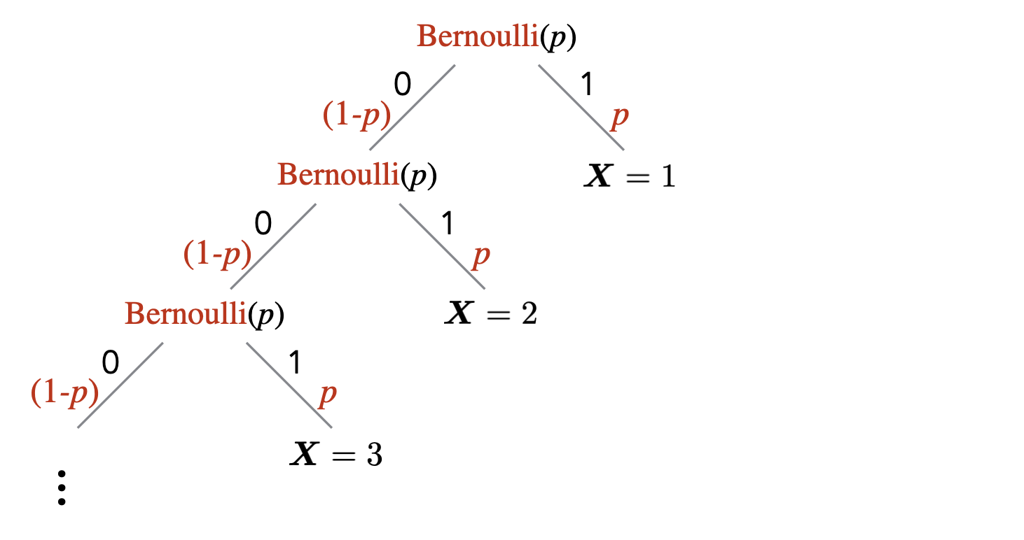
Let \(\mathbf{X}\) be a geometric random variable. Verify that \(\sum_{n = 1}^\infty p_{\mathbf{X}}(n) = 1\).
Recall that for \(|r| < 1\), \(\sum_{n=0}^{\infty}r^n = 1/(1-r)\). Then \[\begin{aligned} \sum_{n=1}^{\infty}p_{{\mathbf{X}}}(n) = \sum_{n=1}^{\infty}(1-p)^{n-1}p = p \cdot \sum_{n=0}^{\infty}(1-p)^{n} = p \cdot \dfrac{1}{1-(1-p)} = 1.\end{aligned}\]
Suppose we repeatedly flip a coin until we see a heads for the first time. What is the probability that we will flip the coin more than \(5\) times?
Let \(\mathbf{X}\) be the number of flips until we see a heads for the first time. Then \(\mathbf{X} \sim \text{Geometric}(1/2)\). The question asks us to compute \(\Pr[\mathbf{X} > 5]\). We know that the event \(\mathbf{X} > 5\) is equivalent to getting tails in our first 5 flips, which happens with probability \(1/2^5\). Therefore \(\Pr[\mathbf{X} > 5] = 1/2^5\).
Let \(\mathbf{X}\) be a random variable with \(\mathbf{X} \sim \text{Geometric}(p)\). Determine \(\mathbb E[\mathbf{X}]\).
By the definition of expectation, we have \(\mathbb E[\mathbf{X}] = \sum_{n=1}^\infty n \cdot (1-p)^{n-1} p\). Using the fact that \(\sum_{n = 0}^\infty (1-p)^n = 1/p\), we get: \[\begin{aligned} \mathbb E[\mathbf{X}] & = \sum_{n=1}^\infty n \cdot (1-p)^{n-1} p \\ & = p \left( \sum_{n=1}^\infty n \cdot (1-p)^{n-1} \right) \\ & = p \left( \sum_{n=1}^\infty (1-p)^{n-1} + \sum_{n=2}^\infty (1-p)^{n-1} + \sum_{n=3}^\infty (1-p)^{n-1} + \cdots \right) \\ & = p \left( \frac{1}{p} + \frac{1-p}{p} + \frac{(1-p)^2}{p} + \cdots \right) \\ & = 1 + (1-p) + (1-p)^2 + \cdots \\ & = \frac{1}{p}.\end{aligned}\]
Here are some general tips on probability calculations (this is not meant to be an exhaustive list).
If you are trying to upper bound \(\Pr[A]\), you can try to find \(B\) with \(A \subseteq B\), and then bound \(\Pr[B]\). Note that if an event \(A\) implies an event \(B\), then this means \(A \subseteq B\). Similarly, if you are trying to lower bound \(\Pr[A]\), you can try to find \(B\) with \(B \subseteq A\), and then bound \(\Pr[B]\).
If you are trying to upper bound \(\Pr[A]\), you can try to lower bound \(\Pr[\overline{A}]\) since \(\Pr[A] = 1-\Pr[\overline{A}]\). Similarly, if you are trying to lower bound \(\Pr[A]\), you can try to upper bound \(\Pr[\overline{A}]\).
If you need to calculate \(\Pr[A_1 \cap \cdots \cap A_n]\), try the chain rule. If the events are independent, then this probability is equal to the product \(\Pr[A_1] \cdots \Pr[A_n]\). Note that the event “for all \(i \in \{1,\ldots,n\}\), \(A_i\)” is the same as \(A_1 \cap \cdots \cap A_n\).
If you need to upper bound \(\Pr[A_1 \cup \cdots \cup A_n]\), you can try to use the union bound. Note that the event “there exists an \(i \in \{1,\ldots,n\}\) such that \(A_i\)” is the same as \(A_1 \cup \cdots \cup A_n\).
When trying to calculate \(\mathbb E[\mathbf{X}]\), try:
directly using the definition of expectation;
writing \(\mathbf{X}\) as a sum of indicator random variables, and then using linearity of expectation.
Describe what a probability tree is.
True or false: If two events \(A\) and \(B\) are independent, then their complements \(\overline{A}\) and \(\overline{B}\) are also independent. (The complement of an event \(A\) is \(\overline{A} = \Omega \backslash A\).)
True or false: If events \(A\) and \(B\) are disjoint, then they are necessarily independent.
True or false: For all events \(A,B\), \(\Pr[A \; | \;B] \le \Pr[A]\).
True or false: For all events \(A,B\), \(\Pr[\overline{A} \; | \;B] = 1- \Pr[A \; | \;B]\).
True or false: For all events \(A,B\), \(\Pr[A \; | \;\overline{B}] = 1 - \Pr[A \; | \;B]\).
True or false: Assume that every time a baby is born, there is \(1/2\) chance that the baby is a boy. A couple has two children. At least one of the children is a boy. The probability that both children are boys is \(1/2\).
What is the union bound?
What is the chain rule?
What is a random variable?
What is an indicator random variable?
What is the expectation of a random variable?
What is linearity of expectation?
When calculating the expectation of a random variable \(\mathbf{X}\), the strategy of writing \(\mathbf{X}\) as a sum of indicator random variables and then using linearity of expectation is quite powerful. Explain how this strategy is carried out.
True or false: Let \(\mathbf{X}\) be a random variable. If \(\mathbb E[\mathbf{X}] = \mu\), then \(\Pr[\mathbf{X} = \mu] > 0\).
True or false: For any random variable \(\mathbf{X}\), \(\mathbb E[1/\mathbf{X}] = 1/\mathbb E[\mathbf{X}]\).
True or false: For any random variable \(\mathbf{X}\), \(\Pr[\mathbf{X} \geq \mathbb E[\mathbf{X}]] > 0\).
True or false: For any non-negative random variable \(\mathbf{X}\), \(\mathbb E[\mathbf{X}^2] \le \mathbb E[\mathbf{X}]^2\).
True or false: For any random variable \(\mathbf{X}\), \(\mathbb E[-\mathbf{X}^3] = - \mathbb E[\mathbf{X}^3]\).
What is Markov’s inequality?
What is a Bernoulli random variable? Give one example.
What is the expectation of a Bernoulli random variable, and how do you derive it?
What is a Binomial random variable? Give one example.
What is the expectation of a Binomial random variable, and how do you derive it?
What is a Geometric random variable? Give one example.
What is the expectation of a Geometric random variable (justification not required)?
Let \(\mathbf{X}\) and \(\mathbf{Y}\) be random variables. Does the expression \(\mathbb E[\mathbf{X} \; | \;\mathbf{Y}] = 0\) type-check?
Let \(A\) be an event. Does the expression \(\mathbb E[A] = 0\) type-check?